The logic of consciousness. Part 7. Self-organization of the context space

Earlier we said that any information has both external form and internal meaning. The external form is what we, for example, saw or heard. Meaning is the interpretation we gave it. Both the external form and the meaning can be descriptions composed of certain concepts.

It was shown that if the descriptions satisfy a number of conditions, then they can be interpreted by simply replacing the concepts of the original description with other concepts, applying certain rules.

Interpretation rules depend on the attendant circumstances in which we are trying to interpret the information. These circumstances are called context in which information is interpreted.
')
The cerebral cortex consists of neural minicolumns. We assumed that each crust minicolumn is a computational module that works with its own information context. That is, each zone of the cortex contains millions of independent calculators of meaning, in which the same information receives its own interpretation.

The mechanism of encoding and storing information was shown, which allows each mini-column of the cortex to have its full copy of the memory of all previous events. The presence of its own full memory allows each minicolumn to check how its interpretation of current information is consistent with all previous experience. Those contexts in which the interpretation turns out to be “similar” to something previously familiar form a set of meanings contained in the information.

In one cycle of its work, each zone of the cortex checks millions of possible hypotheses regarding how to interpret the incoming information, and selects the most meaningful of them.

In order for the core to work this way, it is necessary to first form a context space on it. That is, select all those "sets of circumstances" that affect the rules of interpretation.

Our brain originated from evolution. Its general architecture, principles of work, the system of projections, the structure of the zones of the cortex are all created by natural selection and incorporated into the genome. But not everything is possible and it makes sense to pass through the genome. Some knowledge must be acquired by living organisms independently after their birth. The ideal adaptation to the environment is not to hereditarily keep the rules for all occasions, but to learn how to learn and find optimal solutions in any new circumstances.

Contexts are the very knowledge that must be formed under the influence of the external world and its laws. In this part we describe how contexts can be created and how subsequent self-organization can occur already within the context space.

For each type of information, its own "tricks" work, allowing to form a context space. We describe the two most obvious techniques.

Creating contexts with examples

Suppose there is a teacher who gave us some descriptions and showed how to interpret them. At the same time, he did not just give the correct interpretation, but also explained how it was obtained, that is, what concepts were passed on during interpretation. Thus, for each example, we became aware of the rules of interpretation. In order to create contexts from these rules, they should be combined into groups so that, on the one hand, there are as few of these groups as possible, and on the other hand, that the rules within one group do not contradict each other.

For example, you have sentences and their translations into another language. At the same time there are comparisons of what words are translated. For different sentences it may turn out that the same words will be translated differently. The task is to find such semantic areas, they are contexts in which the translation rules will be stable and unambiguous.

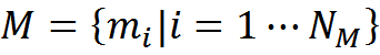
We write this formally. Suppose that we have a memory M , consisting of examples of the form "description - interpretation - transformation rules".




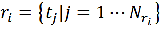
The description and its interpretation are interconnected by the transformation rules r . The rules tell how its interpretation was obtained from the original description. In the simplest case, the transformation rules may simply be a set of rules for replacing some concepts with others.




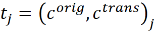
That is, the transformation rules are a set of transformations “source concept - concept-interpretation”. In the more general case, one concept may turn into several or several concepts that may be transformed into one, or one description from several concepts may pass into another complex description.


We introduce the following consistency functions for the two transformation rules. The number of matching transformations


The number of contradictions


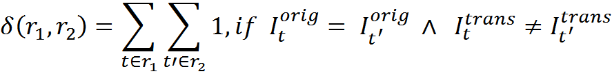
The number of contradictions shows how many transformations are present in which the same source information is transformed by the rules differently.

Now we solve the clustering problem. We divide all memories into a minimal number of classes with the condition that all memories of one class should not contradict each other with their own transformation rules. The resulting classes will be the context space {Cont _i | i = 1 N _Cont }.

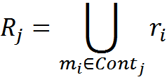
For each context class, we will consider the transformation rules R as a set of all the rules for the elements included in this class.


For the required clustering, you can use the idea of ​​EM (expectation-maximization) algorithm with the addition. The EM algorithm implies that we first break objects into classes in any reasonable way, most often by random assignment. For each class, we consider its portrait, which can be used to calculate the likelihood function of assignment to this class. Then, we redistribute all the elements into classes, based on which class most likely corresponds to each of the elements.

If any element is not plausibly attributed to any of the classes, then create a new class. After assignment to classes, we return to the previous step, that is, we again recalculate the portraits of the classes, in accordance with those who fall into this class. Repeat the procedure until convergence.

In real cases, for example in our life, information does not appear all at once in one go. It accumulates gradually as you gain experience. At the same time, new knowledge is immediately included in the information circulation along with the old ones. It can be assumed that our brain uses two-stage processing of new information. At the first stage, a new experience is remembered and can be immediately used. At the second stage, the correlation of the new experience with the old and more complex joint processing of this processing takes place.

It can be assumed that the first stage occurs during awake and does not interfere with other information processes. The second stage, it seems, requires the “stop” of the main activity and the transition of the brain to a special mode. It seems that such a special regime is sleep.

Proceeding from this, we change a little classical EM algorithm, bringing it closer to the possible push-pull scheme of the brain. We will start with an empty set of classes. We will use the “wakefulness” phase to gain new experience. We will change the portrait of each of the classes immediately after assigning to it a new element. We will use the “sleep” phase to rethink the accumulated experience.

The likelihood function of assigning a memory element with transformation rules r to the context class with number j is chosen


The algorithm will look like:

1. Create an empty classset
   
2. In the “wakefulness” phase, we will consistently submit a new part of the experience.
   
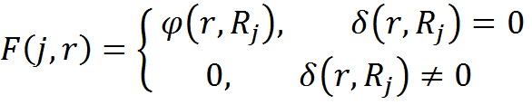
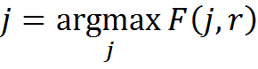
3. We will compare the r component of the elements and the portraits of the classes R. For each element we will choose classes with δ (r, R _j ) = 0 and among them the class with the maximum φ (r, R _j ), which corresponds to
   
   
   
   
   
4. If there are no classes without contradictions, then we will create a new class for such an element and place it there.
   
5. When adding an element to the class, we will recalculate the portrait of the class R.
   
6. Upon completion of the “wakefulness” phase, we proceed to the “sleep” phase. We will reconsolidate the accumulated experience. For the experience obtained during the “wakefulness”, and for a part of the old experience (ideally for all the old experience), we will make a reassignment to the context classes with the creation, if necessary, of the new classes. If we change the assignment of any experience, we will change the portraits of both classes - the one from which the element has dropped out and the one to which it is now assigned.
   
7. We will repeat the “wakefulness” and “sleep” phases, presenting a new experience and reconsolidating the old one.
   

Finding translation rules for fixed contexts

The context creation mechanism described above is suitable for teaching, when the teacher explains the meaning of the phrases and at the same time indicates an interpretation for each of the concepts. Another variant of creating contexts is related to the situation when the contextual transformation is known for teaching examples and there are two informational descriptions corresponding to the initial information and its interpretation. But at the same time, it is not known which of the concepts exactly has passed into.

Such a situation arises, for example, during the training of the primary visual cortex. Fast, abrupt eye movements are called saccades and microsaccades. Before and after the jump, the eye sees the same picture, but in a different context of displacement. If a leap of a certain amplitude and direction is compared with a specific context, then the question will be, according to what rules does any visual description change in this context? Obviously, having a sufficient set of “source picture - picture after offset” pairs related to identical offsets, one can construct a universal set of transformation rules.

Another example. Suppose you want to learn the translation into another language of a word in a specific context. You have a set of sentences, some of which have this word. And there are translations of all these sentences. Pairs "sentence - translation" are pre-divided into contexts. This means that for all translations related to the same context, this word is translated the same way. But you do not know exactly which word in the translations corresponds to what you are looking for.

The task of translation is solved very simply. You need in the context in which the translation is sought to select those pairs of "sentence - translation", in which there is a search word, and see what is common in all translations. This common will be the desired translation of the word.

Formally, it can be written like this. We have a memory M , consisting of memories of the form "description - interpretation - context."




The description and its interpretation are interconnected by the transformation rules R _j , which are unknown to us. But we know the context number Cont _i in which these transformations are made.

Now suppose that in the current description we have met the information fragment I ^orig and we have the context number j in which we want to get an interpretation of this description I ^trans .

Select from memory M a subset of elements M 'such that their contextual transformation coincides with j and in the original description contains a fragment I ^orig , the transformation for which we want to find


In all transformations I ^int _{i there} will be a fragment of the transformation we are looking for (if the context allows such a transformation). Our task is to define such a maximum along the length of the description, which is present in all interpretations of the elements of the set M '.

Interestingly, the ideology of finding such a description coincides with the ideology of algorithms for quantum computing, based on the amplification of the required amplitude. In the descriptions I ^int _{i of the} set M ', all other elements, except the ones sought, are found at random. This means that it is possible to organize the interference of descriptions so that the necessary information is amplified, and the unnecessary interfered randomly and extinguished each other.

To do a “trick” with an amplitude jump, it is required that the data be presented accordingly. Let me remind you that we use a discharged binary code to encode each concept. The description of several concepts corresponds to a binary array, resulting in the logical addition of the binary codes included in the description of the concepts.

It turns out that if we take the binary arrays corresponding to the interpretations and execute an “interference” with them associated with amplifying the code we need, then the result will be a binary code of the transformation we need.

Suppose that M 'contains N elements. Let us match each description with an I ^int bit array of b bits of m, derived from the logical addition of the codes included in the description of the concepts. Create an array of amplitudes A of dimension m


Increasing the number of examples N useful code elements will remain equal to 1 (or will be about 1 if the data contains an error), unnecessary elements will be reduced to a value equal to the probability of a random occurrence of one in the description code. Having cut off the threshold that is guaranteed to exceed the random level (for example, 0.5), we get the desired code.

Correlated contexts

Usually, when determining the meaning of information, it turns out that quite a lot of high values ​​of the correspondence function occur in the context space. This is due to two reasons. The first reason is the presence of several meanings in the information. The second reason is recognition in contexts close to the main one.

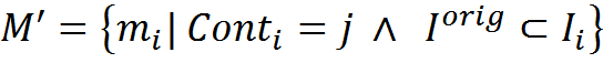
Suppose that reference images of numbers are stored in memory. For simplicity, let us assume that the images in memory are centered and brought to the same scale. Again, for the sake of simplicity, we assume that the figures in the submitted images coincide with the reference ones, but can be in arbitrary locations. In such a situation, the recognition of numbers in the picture is reduced to the consideration of descriptions in different contexts of displacements horizontally and vertically. The context space can be represented as shown in the figure below. Each context, which is indicated by a circle, corresponds to a certain offset applied to the picture in question.


The space of horizontal and vertical offset contexts (the offset is given in arbitrary units)

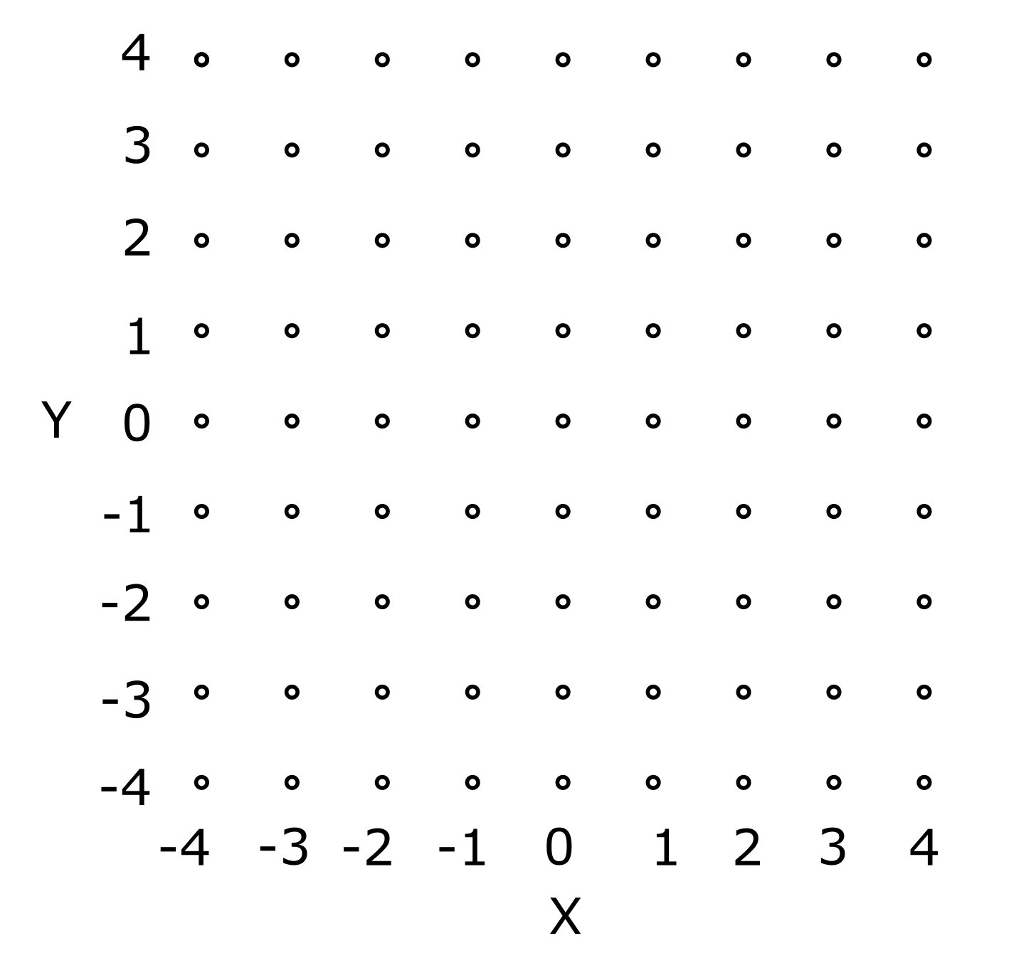
Let's submit an image with two letters A and B (figure below).

Image with two letters

Each of the letters will be recognized in the context that leads it to the corresponding reference stored in memory. In the figure below, the context most suitable for letters is highlighted in red.


Context space. Highlighted contexts with high match function values

But the algorithm for determining compliance can be constructed so that the correspondence, to one degree or another, will be determined not only by exact coincidence, but also by strong similarity of descriptions (such measures will be shown later). Then a certain level of the correspondence function will be not only in the most appropriate contexts, but also in contexts close to them according to the transformation rules. At the same time, proximity does not mean the number of matched rules, but a certain proximity of the descriptions obtained. In the sense that two rules that translate one and the same concept into different but close concepts are two different rules, but at the same time two close transformations. Close contexts are shown in the figure above in pink.

After highlighting the meaning in the original image, we expect to receive a description of the form: the letter A in the context of a shift (2.1) and the letter B in the context of a shift (-2, -1). But for this you need to leave only two main contexts, that is, to get rid of unnecessary contexts. In this case, contexts close in meaning to local maxima, those indicated in the figure above are marked pink, are superfluous.

In determining the meaning, we cannot take the global maximum of the correspondence functions and stop there. In this case, we define only one of the two letters. We can not focus only on a certain threshold. It may happen that the level of compliance in the second local maximum will be lower than the level of contexts surrounding the first local maximum.

In many real-world problems, contexts allow for the introduction of some reasonable proximity measures. That is, for any context, you can specify contexts that are similar to it. In such situations, the full definition of meaning becomes impossible without taking into account this mutual similarity.

In the example above, we did not depict contexts as separate independent entities, but placed them on a plane in such a way that the proximity of the points representing the context became consistent with the proximity of contextual transformations. And then we were able to describe the desired contexts as local maxima on the plane of the points representing contexts. And superfluous contexts have become the closest surroundings of these local maxima.

In general, you can use the same principle, that is, place points on the plane or in multidimensional space corresponding to the contexts so that their proximity best matches the proximity of the contexts. After that, the selection of a set of meanings contained in the information is reduced to the search for local maxima in the space containing points of contexts.

For a number of problems, the proximity of contexts can be determined analytically. For example, for the task of visual perception, the main contexts are geometric transformations, for which the degree of their similarity can be calculated. In artificial models, for some tasks this approach works well, but for biological systems a more universal approach based on self-organization is needed.

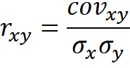
Suppose that by some method we managed to form contexts. Close contexts can be considered such contexts, whose correspondence functions respond in the same way to the same information. Accordingly, the Pearson correlation coefficient between the context matching functions can be used as a measure of context similarity:


For the entire set of contexts, it is possible to calculate the correlation matrix R , whose elements are the pairwise correlations of the matching functions.

Then you can describe the following algorithm for the selection of meanings in the description:

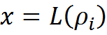
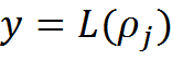
1. In each of the contexts, the original description receives the interpretation and assessment of the correspondence between the interpretation and the memory.
   
2. The global maximum of the correspondence function ρmax and the corresponding maximum context-winner are determined.
   
3. If ρ _max exceeds the cut-off threshold L ₀ , then one of the semantic values ​​is formed, as interpreted in the winning context.
   
4. The activity (the value of the correspondence functions) of all contexts, the correlation with which, on the basis of the matrix R , exceeds a certain threshold L ₁ , is suppressed.
   
5. The procedure is repeated from step 2 until ρmax drops below the cut-off threshold L ₀ .
   

As a result, we get all independent semantic interpretations and get rid of less accurate interpretations, but close to them.

In convolutional neural networks, convolution at different coordinates is analogous to viewing images in various displacement contexts. Using a set of kernels for convolution is similar to having different memories. When a convolution on a nucleus in a certain place shows a high value, in neighboring simple cells responsible for the convolution on the same nucleus in neighboring coordinates, an increased value also occurs, forming a “shadow” around the maximum value. The reason for this “shadow” is similar to the reason for raising the correspondence function in the neighborhood of the context with the maximum value.

To get rid of duplicate values ​​and reduce the size of the network, use the max-pooling procedure. After the layer of convolution, the space of the image is divided into non-intersecting areas. In each region, the maximum value of the convolution is selected. After that, a smaller layer is obtained, where the effect of “shadow” values ​​is significantly weakened due to spatial coarsening.

Spatial organization

The correlation matrix of R determines the similarity of contexts. In our assumptions, the cerebral cortex is located on the plane of a minicolumn, each of which is a processor of a particular context. It seems quite reasonable to place minicolumns not randomly, but so that similar contexts are located as close as possible to each other.

There are several reasons for this placement. Firstly, it is convenient for finding local maxima in the context space. Actually, the very concept of local maximum applies only to a set of contexts that have some kind of spatial organization.

Secondly, it allows to “borrow” interpretations. It may be that the memory of a particular context does not contain an interpretation for any concept. In this case, you can try to use the interpretation of any context that is close in meaning, which has this interpretation. There are other very important reasons, but we'll talk about them later.

The task of placing on a plane, on the basis of similarity, is close to the task of laying a weighted undirected graph. In a weighted graph, edges do not only define connections between vertices, but also determine the weights of these relations, which can be interpreted, for example, as a measure of the proximity of these vertices. The laying of a graph is the construction of such an image of the graph that best conveys the measure of proximity, given by the weights of the edges, through the distance between the vertices of the graph shown.

To solve this problem, a spring analogy is used (Eades P., Congressus Nutnerantiunt - A heuristic for graph drawing drawing, 42, pp. 149–160. 1984.). Connections between vertices are represented by springs. The tension force of the springs depends on the weight of the corresponding edge and the distance between the connected vertices. So that the peaks do not fall into one point, the repulsive force is added, which acts between all the vertices.

For the resulting spring system, we can write the potential energy equation. Energy minimization corresponds to finding the required graph layout. In practice, this problem is solved either by simulating the motion of the vertices under the action of arising forces, or by solving a system of equations arising from recording the energy minimization conditions (Kamada, T., Kawai, S., Information Processing Letters, Vol. 31. - pp. 7-15. - 1989).


,

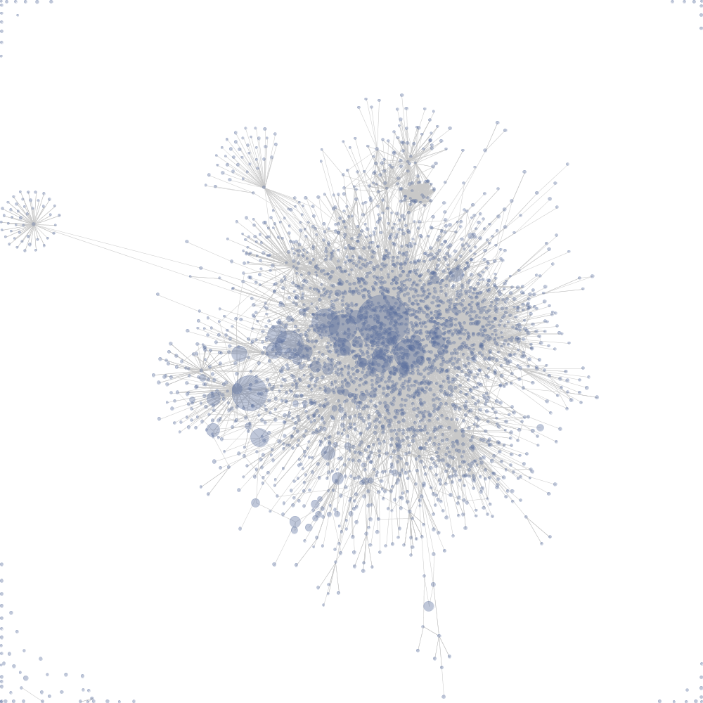
A specific analogue of laying a graph for the case of cellular automata is Schelling's segregation model (The Journal of Mathematical Sociology Volume 1, Issue 2, 1971. Thomas C. Schelling pages 143-186). In this model, the cells of the machine can take values ​​of different types (colors) or be empty. For non-empty cells, the satisfaction function is calculated, which depends on how much the cell environment resembles the cell itself. If the satisfaction is too low, then the value of this cell moves to a free cell. The cycle is repeated until the state of the machine is stabilized. As a result, if the parameters of the system allow it, the initial random disorder is replaced by islands consisting of values ​​of the same type (figure below). Segregation models are used, for example,to simulate the resettlement of people with different incomes, faith, race and the like.




The initial and final state of segregation in four colors

The idea of ​​minimizing the energy of a graph and the principle of segregation of a cellular automaton can be applied with some changes to the spatial organization of contexts. The following algorithm is possible:

1. We define contexts characteristic of the incoming information.
   
2. We determine the matrix of mutual correlations of contexts.
   
3. Randomly distribute contexts to the cells of a cellular automaton, the size of which allows to contain all contexts.
   
4. Select a random cell containing the context.
   
5. We iterate over neighboring cells, for example, the eight nearest neighbors, as a potential place to move the context if the cell is empty, or to exchange contexts if not empty.
   
6. We calculate the change in the energy of the automaton in the case of each of the potential movements (exchanges).
   
7. Make a move (exchange) that best minimizes energy. If this is not, then we remain in place.
   
8. Repeat from step 4 until the state of the machine does not stabilize.
   

As a result, contexts are made so that similar contexts, if possible, are close to each other. You can see how this self-organization happens on the video below.



Each color point on the video corresponds to its context. Each context has several parameters that define it. Context correlation is calculated from the proximity of these parameters. In the given example, there is no creation of contexts from the initial information; it is just an illustration of the spatial organization for the case when correlations between contexts are already calculated in advance. A program illustrating self-organization by the permutation method is available here .

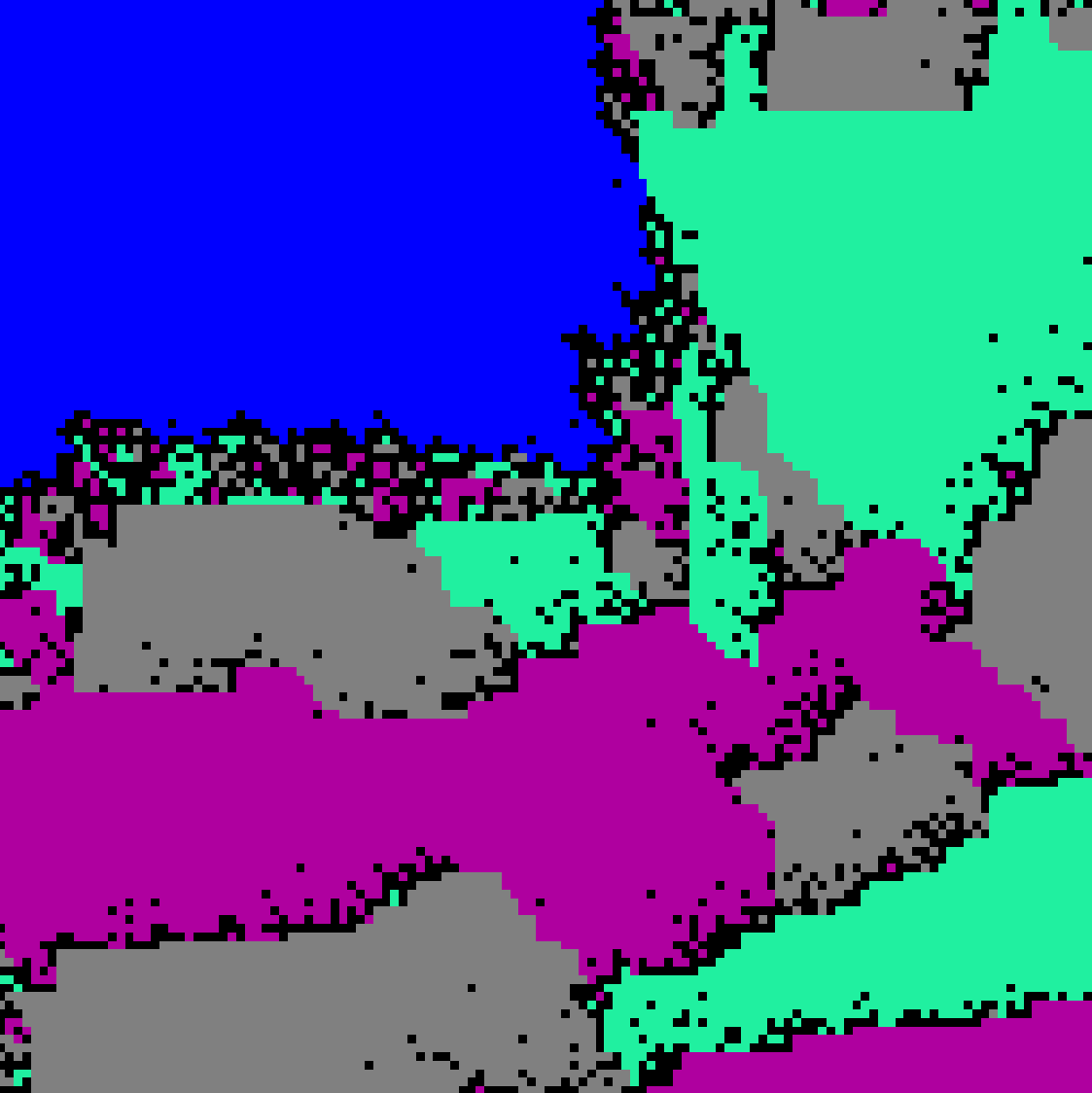
In the above example, the contexts correspond to all possible combinations of the four parameters. The first parameter is circular, two parameters are linear, the fourth takes two values. This corresponds to the contexts that can be used for image analysis. The first parameter describes the rotation, the second and third horizontal and vertical displacements, respectively, the fourth parameter indicates the information to which eye belongs.

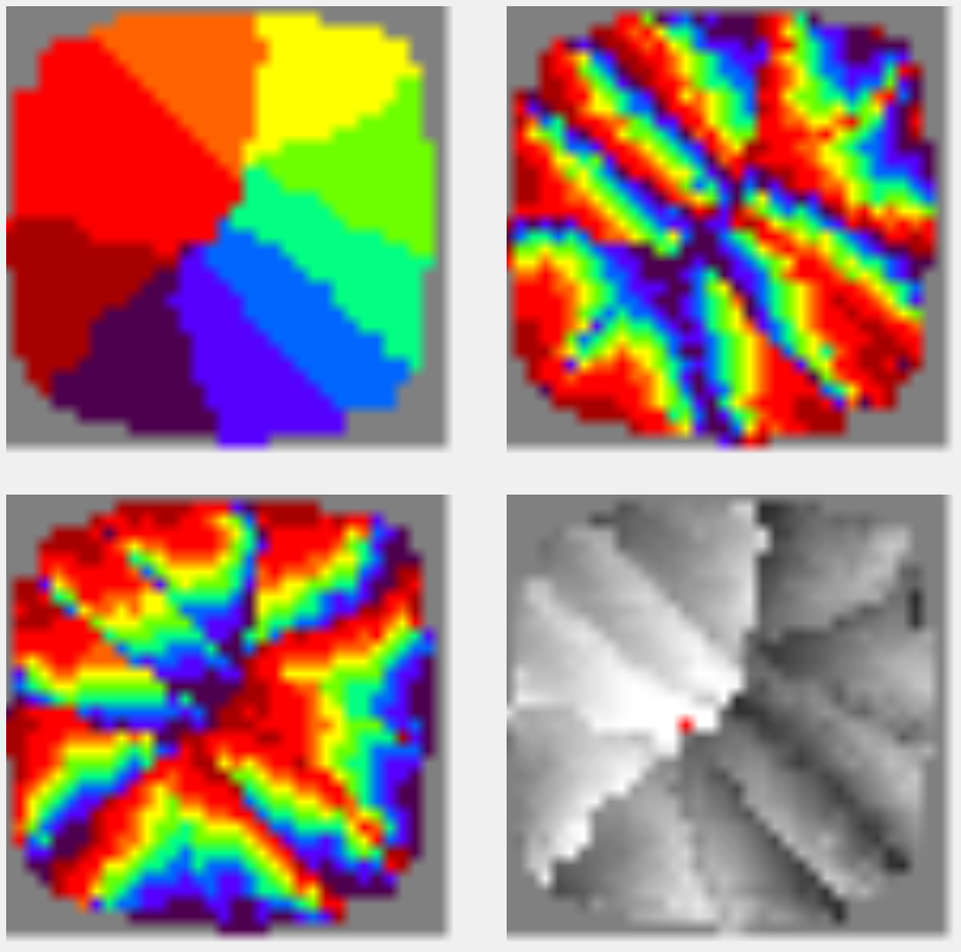
Each parameter is associated with a color spectrum. According to the proximity of colors in the spectrum, one can judge the proximity of the parameter values. In the example, each context has four values. That is, its value for each of the parameters and, accordingly, its color in each of them. The squares show the colors of the contexts in each of the parameters. All color pictures show the same contexts, but in colors of different parameters (figure below).


The result of self-organization for contexts with four independent parameters

The essence of spatial ordering is that the contexts in the process of moving have to find a compromise between all the parameters. In the video example, this compromise is achieved due to the fact that the linear parameters build a linear field. That is, contexts arise in such a way that they form a certain correspondence of the coordinate grid. By the way, this is how the contexts were set on the example above, when we talked about the recognition of letters.

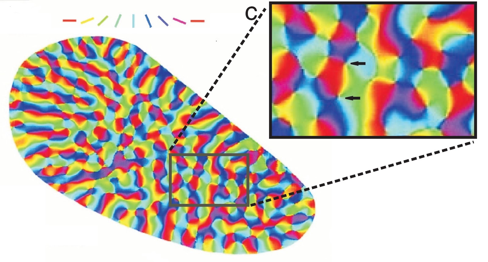
For the ring parameter of rotation over the entire surface, groups were formed that contain a complete set of colors. In the visual cortex, such constructions are called "turntables" or "tops." How do the "turntables" in the primary visual cortex, shown in the title picture. In more detail about it and about the fourth square with columns of an eye-dominance will be told in the following part.

Depending on how many intervals each of the parameters is split, a different number of contexts is obtained, which will certainly be close to each other. If the annular parameter is more fragmented than linear, a picture can be obtained when the contexts are lined up into one big “spinner” (figure below). In this case, the linear parameters will form local linear fields distributed throughout the space.


Spatial organization of contexts for a case with three independent parameters. The ring parameter dominates and forms a global “spinner”; two linear parameters form local linear fields. The lower right square shows elements close to the one highlighted by a red dot.

Regardless of what the permutation process converges to, similar contexts are mostly next to each other. The pictures below show examples of such proximity. In each figure, one of the contexts is highlighted in red, the brightness of the other contexts corresponds to the degree of their proximity to the selected context.


Distribution of the proximity of contexts in relation to the selected

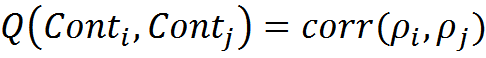
When applying the described algorithm is required to take into account all the mutual correlation of contexts. The correlations themselves can be represented as connections of the cells of the automaton. Each cell is associated with all other cells. Each link is responsible for the pairwise correlation of those cells between which it passes. You can significantly reduce the number of connections if you use the Barnes-Hut method(Barnes J., Hut P., A hierarchical O (N log N) force-calculation algorithm. Nature, 324 (4), December 1986). Its essence lies in replacing the influence of remote elements on the influence of quadrants, including these elements. That is, remote elements can be combined into groups and treated as one element with the average distance for the group and the average bond strength. This method works especially well for calculating the mutual attraction of stars in star clusters .


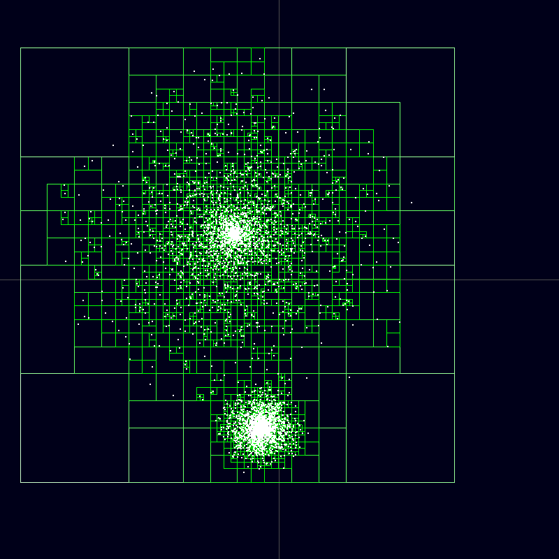
Spatial quadrants replacing individual stars

With a similarly organized map of contexts, it is possible to somewhat simplify the solution of the problem of searching for local maxima. Now each context needs to be connected with other similar contexts located close to it, and with islands of similar contexts, taken for some distance. The length of such connections after spatial organization will be less than before the organization, since it is this criterion that was the basis for calculating the energy of the system.

The benefits of spatial organization

Let's go back to the translation example. Contests are semantic areas in which general translation rules apply. Having placed the contexts spatially, we get the neighboring groups of contexts related to approximately the same subject. Within the group, each of the individual contexts expresses the subtleties of the translation in a certain specified sense.

How many contexts do you need? It would seem, the more the better. The more contexts available, the more details and shades of meaning can be taken into account when choosing a translation. But the flip side of the detail is the fragmentation of the interpretation experience. In order to know the translation rules for any words in a specific context, one must have experience in their translation in this particular context. Each translation example gives us a set of translation rules. If these rules are attributed to any one context that turned out to be the most successful, they will be inaccessible to other contexts.

Spatial organization and correlation links allow for any selected context to understand which contexts are close to him in meaning. This means that if there is no own translation experience in the selected context, you can use the experience of translating neighboring contexts of similar meaning, if such experience is there.

Appeal to the experience of neighbors allows you to search for a compromise between detalization of contexts and fragmentation of experience. For translation, it may look like a group of contexts related to general topics and located close to each other, jointly store the translation rules for this subject area. In addition, each separate context contains certain own clarifications that reflect the nuances of meaning.

In addition, the limited number of available contextual modules in real-world problems will require finding the best approximate solution. This can be greatly helped by the fact that the spatial context map itself largely takes into account the specifics of the information being processed.

Another benefit of spatial organization is the ability to "do several things at the same time." The conversation does not mean that we can, for example, simultaneously drive a car and talk on the phone. If different bark zones are involved for this, then there is nothing surprising in this. But everything becomes more interesting when we have to talk with someone and think about something of our own, or talk at once on two different topics with different interlocutors, or, like Caesar, write and simultaneously speak on another topic. It turns out that the same areas of the cortex are forced to work simultaneously with several information flows.

Probably, everyone noticed on himself that it was possible to combine things or thoughts only when they differed quite strongly in meaning. As soon as the meaning begins to intersect, confusion begins, or one thought completely supersedes the other.

In our model, the combination of information flows can be explained by their separation in the space of contexts. While each of the meanings is processed in its place, nothing terrible happens. The convergence of meanings and, accordingly, contexts makes the combination impossible.

In practice, with the convergence of meanings, the so-called “brain overload” can occur, when a person falls into a trance state, loses his own thought and ceases to control himself. The so-called “gypsy hypnosis” is based on this effect.

If several people begin to say something different at the same time, most likely it will not make a special impression on you. Most likely, you will concentrate on someone and you will follow his thought. Trying to hear everyone at the same time is unlikely to give something. You will hear fragments of phrases and most likely give up this activity.

But when you are surrounded by a crowd of gypsies, the situation changes. You are alert and trying to control the situation. You try to understand everything you are told. As a rule, all Roma "beat" in one topic. The "center" gypsy begins to talk about your future, prophesy, warn or threaten. The rest echo her and say something consonant. At this point, most people have a trance. Waking up outside the gypsy environment, a person discovers the loss of a wallet, hours, and confidence in his own normality.

Adaptive calculation of correlations. The role of synaptic plasticity

In the process of spatial organization and at the very definition of meaning, one needs to know the mutual similarity of contexts, which can be determined through the correlation of the activity of the correspondence functions. Correlation analysis is based on the assumption that a random process is stationary over time, that is, averaging over a set of realizations is equivalent to time averaging. Since obtaining new experience changes the contexts themselves, and therefore their correspondence functions, it turns out that it is reasonable not to use the entire set of observations for calculating correlations, but to proceed only from their relatively recent part. Such an approach, in particular, is used in economics for short-term adaptive forecasting of time series, when regularities may have a local temporal character.

To calculate the correlation, which takes into account mainly the last N active observations, you can use an adaptive scheme. We introduce the cut-off threshold L ₀ and the threshold function:


When a new experience arises, we will change the correlation between two contexts only if at least one of them has the compliance function overcoming the threshold L ₀ . If both functions have crossed the threshold, then we will increase the correlation, if only one, then decrease.

For convenience of recording, we introduce a small value:


Pearson correlation is calculated by the formula:


Each of the elements involved in the calculation can be adaptively recalculated when a new experience appears. For matching functions of contexts with numbers i and j, you can write



If at least one of the values, x or y, is non-zero, then we recalculate


Such a correlation will tend to unity if contexts are always activated together and to zero when the process is random. In accordance with this adaptive calculation, weights of the links connecting the contexts can be formed.

Synaptic plasticity

Strengthening the strength of the connection between contexts at the time of their joint operation is very similar to Hebb's rule (Hebb DO - The Organization of Behavior. John Wiley & Sons, New York, 1949). In accordance with it, neurons, triggered together, increase the strength of the connection between them.

If a formal neuron works as a linear adder, then its output is the weighted sum of its inputs.


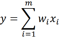
Hebb's rule for such a neuron is


Where n is a discrete time step, and η is the learning speed parameter.

With such training, the weights of those inputs to which the signal x _i (n) is applied increase , but this is done the more strongly the more active is the reaction of the neuron itself (y).

With the direct application of the Hebbian rule, the neuron weights grow indefinitely. This is easily avoided if you require that the total amount of weights of each neuron remain constant. Then, instead of increasing weights, they will be redistributed. Some weights will increase by decreasing others.

Given the general normalization of weights, the Hebbian learning rule takes the form of the Oja learning rule (Oja, 1982)


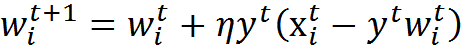
In this formula, x _i ^t is the state of the inputs of the neuron, w _i ^t are the synaptic weights of the neuron, and y ^t is the activity of its output, obtained by weighted summation of the inputs.

The above-described correlation and formal neuron learning outwardly correspond to the principle of enhancing the connections of neurons that work together, but they also implement completely different mechanisms. In the classical Hebbovs training, due to the weighted summation of the signals of the inputs and the subsequent joint normalization of the weights, a redistribution of the weights of the neuron arises in such a way that it is tuned to a specific characteristic stimulus. In our model, nothing like this happens. The essence of correlation weights is the description of the picture of the proximity of contexts in their spatial environment. Weights are trained independently of each other and this has nothing to do with any characteristic stimulus. There is also no requirement for normalization: restricting the growth of weights is a natural consequence of the limited correlation coefficients.

For the real brain, synaptic plasticity is known. Its essence is that the effectiveness of synaptic transmission is not constant and may vary depending on the pattern of current activity. Moreover, the duration of these changes can vary greatly and be caused by different mechanisms.


Dynamics of changes in synaptic sensitivity. (A) - Facilitation, (B) - Strengthening and depression, (C) - post-tetanic potency, (D) - long-term potency and long-term depression (Nicolls J., Martin R., Wallace B., Fuchs P., 2003)

A short volley of spikes can cause relief (facilitation) of the selection of a mediator from the corresponding presynaptic terminal. Facilitation appears instantly, is preserved during a volley, and is substantially noticeable for another 100 milliseconds after the end of stimulation. The same short exposure can lead to the suppression (depression) of the release of a neurotransmitter lasting several seconds. Facilitation can go to the second phase (gain), with a duration similar to the duration of the depression.

A long high-frequency pulse train is usually called tetanus. The name is connected with the fact that this series precedes tetanic muscle contraction. Receipt of tetanus at the synapse, can cause the post-tetanic potency of the release of a mediator, observed for several minutes.

Repeated activity can cause long-term changes in synapses. One of the reasons for these changes is an increase in calcium concentration in the postsynaptic cell. A strong increase in concentration triggers a cascade of secondary mediators, which leads to the formation of additional receptors in the postsynaptic membrane and an overall increase in receptor sensitivity. A weaker increase in concentration has the opposite effect - the number of receptors decreases, their sensitivity decreases. The first condition is called long-term potency, the second - long-term depression. The duration of such changes is from several hours to several days (Nicolls J., Martin R., Wallace B., Fuchs P., 2003).

When Donald Hebb formulated his rule, very little was known about the plasticity of synapses. When the first artificial neural networks were created, they used the idea of ​​the possibility of synapses to change their weights as the key one. It is the smooth adjustment of the scales that allowed neural networks to adapt to the incoming information and to highlight in it any common properties. The grandmother's neuron, which I constantly refer to, is a direct consequence of the idea of ​​tuning synaptic weights to a characteristic stimulus.

Later, when the plasticity of real synapses became better studied, it turned out that it had little in common with the rules for learning neural networks. First, in most cases, changes in the efficiency of synaptic transmission pass without a trace after a short time. Secondly, there is no noticeable consistency in learning various synapses, that is, nothing to remind joint normalization. Thirdly, the efficiency of transmission changes under the action of incoming signals from the outside and it is not very clear how it depends on the reaction of the postsynaptic, that is, the signal receiving neuron. Add to this that, besides all that, real neurons do not work as linear or threshold adders.

The result was an interesting situation. Neural networks work and show good results. Many who are well versed in neural networks, but far from biology, believe that artificial neural networks are in many ways similar to the brain. This concept of similarity is based on the history of the emergence of artificial neural networks and, accordingly, on those ideas about neurons that existed once upon a time. Those researchers who are better at brain biology prefer to say that many ideas of artificial neural networks are inspired by the mechanisms of the real brain. However, one should be aware of the extent of this “instilling”.

My constant return to grandmother's neurons is largely due to attempts to show the difference in understanding the role of synaptic plasticity in the classical approach and in the proposed model. In the classical model, the change in the weights of synapses is the mechanism for tuning neurons to a characteristic stimulus. I believe that the role of synapse plasticity is quite different. It is possible that synaptic plasticity in the neurons of the real brain is partly due to the mechanisms for setting contextual correlations.

Difference of context maps from Kohonen maps

Spatial organization in neural networks is usually associated with self-organizing Kohonen maps (T. Kohonen, Self-Organizing Maps).



Suppose we have input information given by the vector x . There is a two-dimensional lattice of neurons. Each neuron is connected with the input vector x , this connection is determined by the set of weights w _j . Initially, we initiate a network of random small weights. By supplying an input signal, for each neuron one can determine its level of activity as a linear adder. Take the neuron that will show the most activity, and call it the winning neuron. Next, move its weight in the direction of the image, which he was like. Moreover, we will do the same procedure for all its neighbors. We will relax this shift as we move away from the winning neuron.


Here η (n) is the learning rate, which decreases with time, h is the amplitude of the topological neighborhood (dependence on n assumes that it also decreases with time).

The amplitude of the neighborhood can be selected, for example, by the Gaussian function:


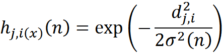
Where d is the distance between the corrected neuron j and the winning neuron i .


Gauss function

As you learn on such a self-organizing map, zones will be allocated corresponding to how the training images are distributed. That is, the network itself will determine when similar pictures will meet in the input stream, and will create for them close representations on the map. At the same time, the more the images will differ, the more separate their representations will be located apart from each other. As a result, if we appropriately color the learning result, it will look something like the one shown in the figure below.


Kohonen Card Learning Result

The result of learning a Kohonen map after coloring may turn out to be similar in appearance to the arrangement of contexts obtained by rearranging them. This similarity should not be misleading. It is about different things. Kohonen maps are based on adapting the weights of neurons to the indicative descriptions given. This, in fact, all the same "grandmother's neurons." The supplied information "sculpts" from neurons detectors of some average "grandmothers". In the centers of the colored areas, “grandmothers” are more or less similar to something, closer to the borders of the regions are “grandmother-mutants”. There are hybrids of neighboring "grandmothers", "grandfathers", "cats" and "dogs".

When you try to try Kohonen maps to the real brain, a significant problem arises. This is the well-known dilemma of "stability-plasticity." The new experience changes the portraits of "grandmothers", forcing all the neighbors of the "grandmother-winner" to change in her direction. As a result, the network can change its organization, erasing previously acquired knowledge. To stabilize the network, the learning rate has to be reduced with time. But this leads to the "ossification" of the network and the inability to continue learning. In our self-organization, the rearrangement of contexts does not violate their integrity. Contexts are moved to a new location, but at the same time, all information stored in them is kept intact.

In the next part I will talk about spatial self-organization in the real crust and try to show that much of what is observed experimentally can be explained precisely in our model.

Alexey Redozubov

The logic of consciousness. Introduction
The logic of consciousness. Part 1. Waves in the cellular automaton
The logic of consciousness. Part 2. Dendritic waves
The logic of consciousness. Part 3. Holographic memory in a cellular automaton
The logic of consciousness. Part 4. The secret of brain memory
The logic of consciousness. Part 5. The semantic approach to the analysis of information
The logic of consciousness. Part 6. The cerebral cortex as a space for calculating meanings.
The logic of consciousness. Part 7. Self-organization of the context space
The logic of consciousness. Explanation "on the fingers"
The logic of consciousness. Part 8. Spatial maps of the cerebral cortex
The logic of consciousness. Part 9. Artificial neural networks and minicolumns of the real cortex.
The logic of consciousness. Part 10. The task of generalization
The logic of consciousness. Part 11. Natural coding of visual and sound information
The logic of consciousness. Part 12. The search for patterns. Combinatorial space