ROAD audio codec analysis
Not so long ago, in Habré, in the article “Application of nonlinear dynamics and Chaos theory to the task of developing a new audio data compression algorithm,” a fundamentally new audio codec with five unique properties never seen before was announced. Such a formulation aroused interest and a desire to understand a little what was happening.
Next will be considered the declared unique properties and made several test measurements.
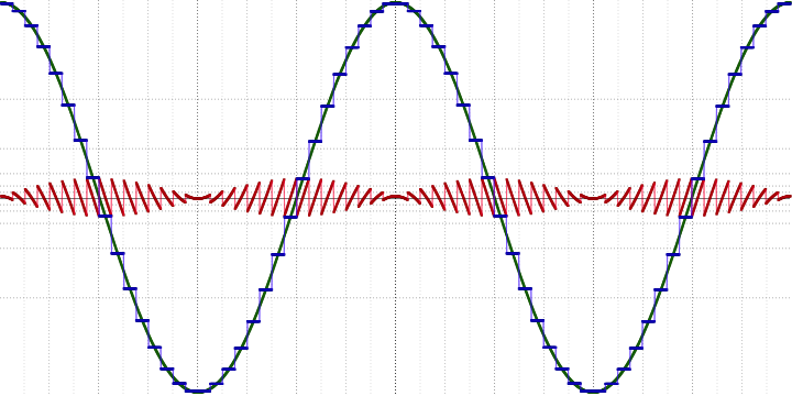
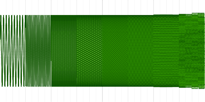
The article describes a rather complicated formula for explaining this property, but in fact everything is much simpler. In fact, this property means that not all of the signal is subjected to compression, but only a part of it, as shown in the following image:
')
Here, the source signal is marked in green, in blue - averaged over a certain number of points (samples) and stored in an explicit form, and in red - the remainder subjected to compression.
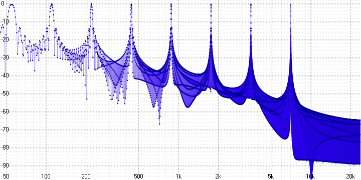
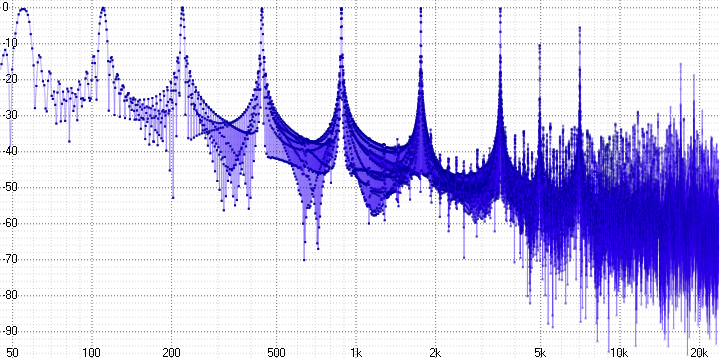
In a very rough approximation, we can say that only the high-frequency part of the signal is compressed. More precisely, in the frequency domain, the division into averaged and residual signals will look, for example, like this (for 4-fold averaging at 48 kHz):
Or so (for 32-fold averaging at 48 kHz):

An even more accurate view will depend on the particular signal taken. For example, for a sine wave from the very first image:
Here averaging has led to the appearance of harmonics in antiphase in both signals, which are mutually compensated with addition. It is obvious that when the phase or amplitude of the harmonic changes in one of the signals (for example, as a result of compression), full compensation will no longer occur and will lead to a distortion of the original signal. Further it will be shown on specific measurements.
This property clearly follows from the previous one. Since part of the signal is stored without compression, it can be reproduced by ignoring the encoded part. The author presents this as a virtue, but it looks extremely dubious. If you downloaded an audio file that is not played by the player, it is clear that some codec is missing. But if the file is played with degraded quality, then it is more logical to assume that it should be so or it is damaged, than to search for a codec that improves its sound.
This word the author called the possibility of resampling (resampling) at the decoder level. This could be called an advantage if it would lead to any significant advantages over the use of other resamplers, including those built into software audio players or audio output devices.
The quality of the resampler is determined by the degree of suppression of parasitic harmonics outside the original frequency band. Further it will be shown that this codec does not possess such quality.
And here already there is an obvious juggling of facts. When digitizing an audio signal, it is not just a decrease in the dynamic range that occurs - quantization noise appears, which are non-linear in nature. They are quite difficult to filter, so in practice they are simply masked by dithering and noise shaping techniques.
It is impossible to recover lost information by any means in order to ensure the declared expansion of the dynamic range. The fact that new samples of the audio stream will be synthesized in the extended range only means the absence of new quantization noise - and only at the processing stage, since the audio playback device also has limited accuracy. And besides, absolutely all resamplers have this property.
Based on the description, one would assume that each time after decoding, we get a slightly different result. However, a real comparison showed that the results are identical. This means that, in fact, this property does not matter - with the same success one can see non-determinism in the order in which to add the numbers 2 and 3 to get the number 5.
The article has an image of Lena, but there is not a single waveform. We will fill this gap in the context of consideration of distortions introduced by a codec.
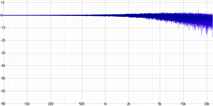
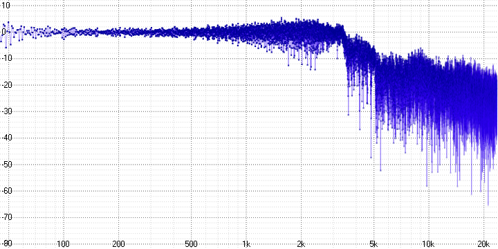
For the measurement, the synthesized signals with a duration of 65,536 samples will be used (for the convenience of subsequent Fourier analysis). The measurement results will be presented both in the time (green) and frequency (blue) areas in the form of a logarithmic amplitude-frequency characteristic.
When encoding used the following parameters:
This is a standard tool for carrying out such measurements. In appearance and hearing it looks like white noise with the only difference being that it is limited for a given period of time and has a discrete character. For audio measurements, it is usually formed through the inverse Fourier transform, in which all amplitudes equate to a constant, and phases to pseudo-random values.
After measuring by the form of the frequency response, it is possible to estimate the system response at each individual frequency by the deviation of its amplitude from 0 dB.
Since analyzing noise for distortions in the time domain is rather problematic, here the measurement results will be presented only in the frequency domain.
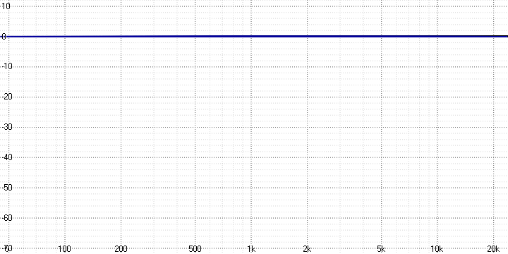
Source signal:
Measurement results:
sample length = 4:
sample length = 8:
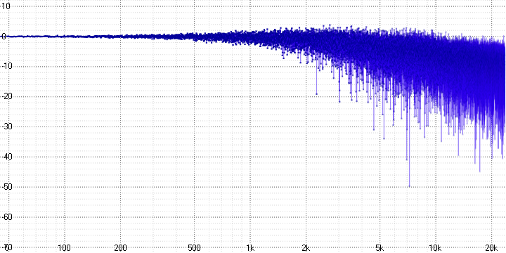
sample length = 16:
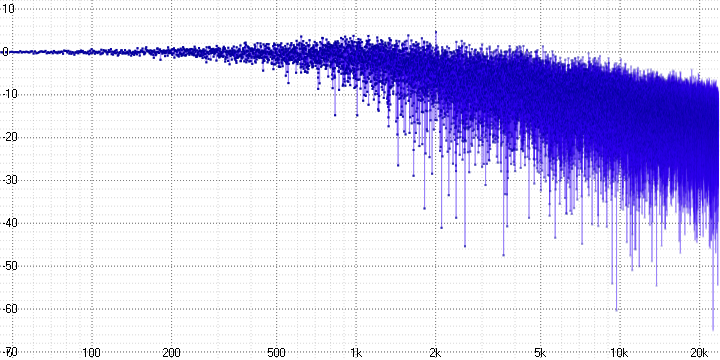
sample length = 32:
Here, the decay and strong noise at high frequencies, which increase with the sample length parameter (which probably determines the number of averaged points), are clearly visible.
It is a sinusoid with a constantly increasing or decreasing frequency.
Here, with decreasing frequency, the amplitude decreases to compensate for the slope of the frequency response (this is not required in a linear sweep tone), and a smoothing window is imposed.
It is often used to evaluate nonlinear distortion (besides distortion) in addition to the frequency response. Here we will not consider any coefficients, but simply evaluate the result visually.
Source signal:

Measurement results:
sample length = 4:
sample length = 8:
sample length = 16:

sample length = 32:
The oscillogram clearly shows that some of the high-frequency information is lost, and the greater the compression ratio, the stronger.
At the frequency response at the same time, it is clear that it is not just lost - it is replaced by harmonics (which inevitably arise when decimating by averaging) and noise.
On the oscillogram you can also see the distortion of the opposite nature - the appearance of sound where it was not. It is difficult to say whether this is a mistake or a feature of the algorithm.
Contains notes “la” from controcade (55 Hz) to “la” of the fifth octave (7040 Hz).
Source signal:

Measurement results:
sample length = 4:
sample length = 8:
sample length = 16:
sample length = 32:
Here we can already unequivocally state the presence of pronounced harmonic distortion. Since a sinusoid is a pure tone, any distortion of it leads to the appearance of harmonics - they are clearly visible (at a frequency of 5 kHz in the first graph, for example).
Consider a sine wave with a frequency of 440 Hz from the last measurement a little closer:
Here you can see that it is assembled from pieces from other sinusoids. Also clearly visible and tears at the edges of the blocks.
In the decoder it is possible to increase the sampling rate by 2 or 4 times and the quantization depth up to 24 bits. Let's test this possibility on the previous signal (with the parameter sample length = 4):

The shape of the signal shows that it has undergone even greater distortion. By frequency response it can be seen that the extended frequency range is filled with noise. Nothing like an expansion of the dynamic range is also observed (for example, in the form of noise reduction).
Of course, from the above graphs it does not at all follow that this codec cannot be used in practice. It is possible that for someone the words “Fractal Compression” and “Chaos Theory” will have much more weight than some kind of graphics. It is equally possible that someone will perceive his distortions as special and pleasant to the ear, which only improve the sound.
But to me personally, the idea of fractal compression as such seems to be far-fetched since the beginning of its appearance and seems to be a kind of “Holy Grail”. Indeed, since the release of the Fractal Geometry of Nature, nothing particularly new has appeared - the same fractal leaves and trees, the Maldebrot and Julia sets, the Koch, Hilbert, Peano curves and the Sierpinski triangles (and the original article did not become an exception in this regard). Moreover, they all have an exclusively geometric nature - no one has yet declared the existence of “audio fractals” endowed with the properties of self-similar sets with fractional metric dimension.
Next will be considered the declared unique properties and made several test measurements.
Property Overview
Pre-listening
The article describes a rather complicated formula for explaining this property, but in fact everything is much simpler. In fact, this property means that not all of the signal is subjected to compression, but only a part of it, as shown in the following image:
')
Here, the source signal is marked in green, in blue - averaged over a certain number of points (samples) and stored in an explicit form, and in red - the remainder subjected to compression.
In a very rough approximation, we can say that only the high-frequency part of the signal is compressed. More precisely, in the frequency domain, the division into averaged and residual signals will look, for example, like this (for 4-fold averaging at 48 kHz):
Or so (for 32-fold averaging at 48 kHz):
An even more accurate view will depend on the particular signal taken. For example, for a sine wave from the very first image:
Here averaging has led to the appearance of harmonics in antiphase in both signals, which are mutually compensated with addition. It is obvious that when the phase or amplitude of the harmonic changes in one of the signals (for example, as a result of compression), full compensation will no longer occur and will lead to a distortion of the original signal. Further it will be shown on specific measurements.
Partial compatibility
This property clearly follows from the previous one. Since part of the signal is stored without compression, it can be reproduced by ignoring the encoded part. The author presents this as a virtue, but it looks extremely dubious. If you downloaded an audio file that is not played by the player, it is clear that some codec is missing. But if the file is played with degraded quality, then it is more logical to assume that it should be so or it is damaged, than to search for a codec that improves its sound.
Overclocking
This word the author called the possibility of resampling (resampling) at the decoder level. This could be called an advantage if it would lead to any significant advantages over the use of other resamplers, including those built into software audio players or audio output devices.
The quality of the resampler is determined by the degree of suppression of parasitic harmonics outside the original frequency band. Further it will be shown that this codec does not possess such quality.
Expansion of dynamic range
And here already there is an obvious juggling of facts. When digitizing an audio signal, it is not just a decrease in the dynamic range that occurs - quantization noise appears, which are non-linear in nature. They are quite difficult to filter, so in practice they are simply masked by dithering and noise shaping techniques.
It is impossible to recover lost information by any means in order to ensure the declared expansion of the dynamic range. The fact that new samples of the audio stream will be synthesized in the extended range only means the absence of new quantization noise - and only at the processing stage, since the audio playback device also has limited accuracy. And besides, absolutely all resamplers have this property.
Non-deterministic decoding
Based on the description, one would assume that each time after decoding, we get a slightly different result. However, a real comparison showed that the results are identical. This means that, in fact, this property does not matter - with the same success one can see non-determinism in the order in which to add the numbers 2 and 3 to get the number 5.
Test on test data
The article has an image of Lena, but there is not a single waveform. We will fill this gap in the context of consideration of distortions introduced by a codec.
For the measurement, the synthesized signals with a duration of 65,536 samples will be used (for the convenience of subsequent Fourier analysis). The measurement results will be presented both in the time (green) and frequency (blue) areas in the form of a logarithmic amplitude-frequency characteristic.
Just in case
Amplitude change of 3 dB is approximately equal to a change of 1.4 times.
Amplitude change of 6 dB is approximately equal to a change of 2 times.
A change in amplitude of 12 dB is approximately equal to a change of 4 times.
Amplitude change of 6 dB is approximately equal to a change of 2 times.
A change in amplitude of 12 dB is approximately equal to a change of 4 times.
When encoding used the following parameters:
- Maximum sample length of rang = from 4 to 32, for each individual measurement was made;
- Length of encoding superframe = 8 (when using the default value, 10, the file was not completely processed and cut off along the right border);
- Relative shifting between domains = 1 (by default).
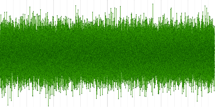
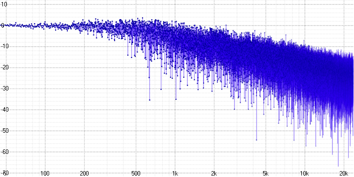
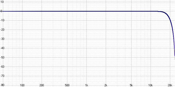
MLS - Maximum Length Sequence
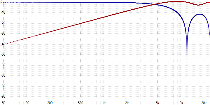
This is a standard tool for carrying out such measurements. In appearance and hearing it looks like white noise with the only difference being that it is limited for a given period of time and has a discrete character. For audio measurements, it is usually formed through the inverse Fourier transform, in which all amplitudes equate to a constant, and phases to pseudo-random values.
After measuring by the form of the frequency response, it is possible to estimate the system response at each individual frequency by the deviation of its amplitude from 0 dB.
Since analyzing noise for distortions in the time domain is rather problematic, here the measurement results will be presented only in the frequency domain.
Source signal:
Measurement results:
sample length = 4:
sample length = 8:
sample length = 16:
sample length = 32:
Here, the decay and strong noise at high frequencies, which increase with the sample length parameter (which probably determines the number of averaged points), are clearly visible.
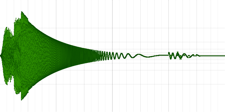
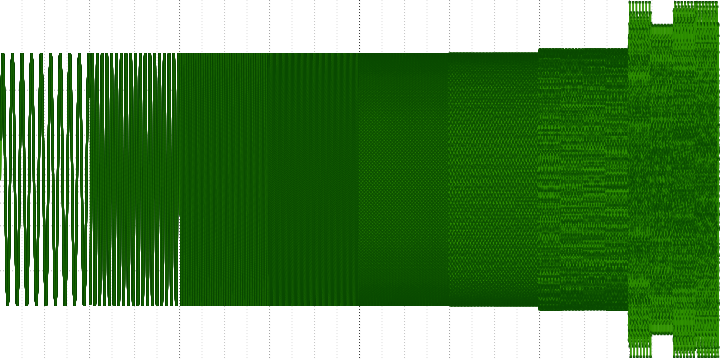
Logarithmic sweep-tone
It is a sinusoid with a constantly increasing or decreasing frequency.
Here, with decreasing frequency, the amplitude decreases to compensate for the slope of the frequency response (this is not required in a linear sweep tone), and a smoothing window is imposed.
It is often used to evaluate nonlinear distortion (besides distortion) in addition to the frequency response. Here we will not consider any coefficients, but simply evaluate the result visually.
Source signal:
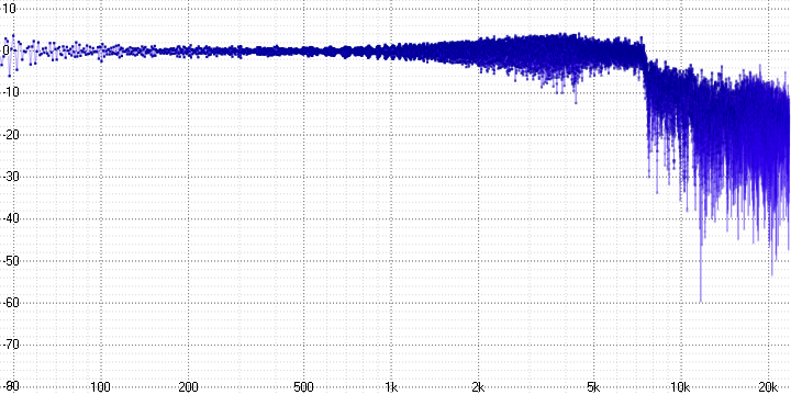
Measurement results:
sample length = 4:
sample length = 8:
sample length = 16:
sample length = 32:
The oscillogram clearly shows that some of the high-frequency information is lost, and the greater the compression ratio, the stronger.
At the frequency response at the same time, it is clear that it is not just lost - it is replaced by harmonics (which inevitably arise when decimating by averaging) and noise.
On the oscillogram you can also see the distortion of the opposite nature - the appearance of sound where it was not. It is difficult to say whether this is a mistake or a feature of the algorithm.
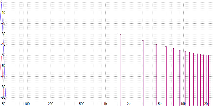
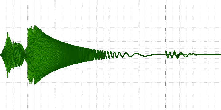
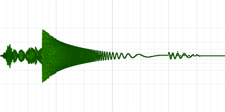
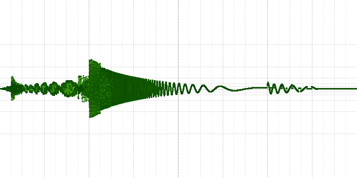
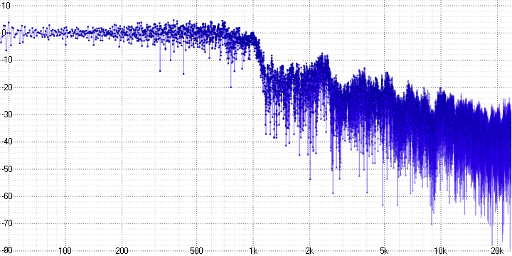
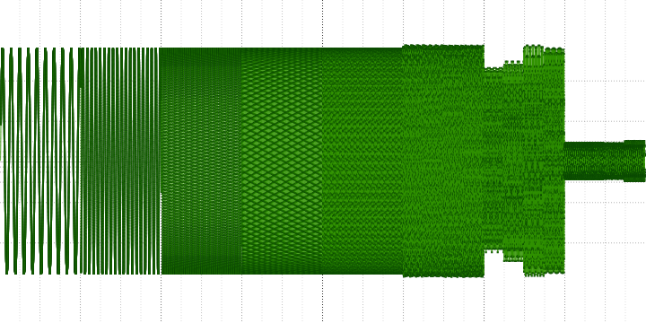
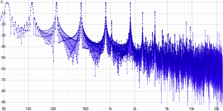
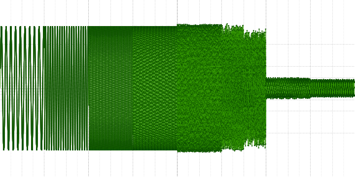
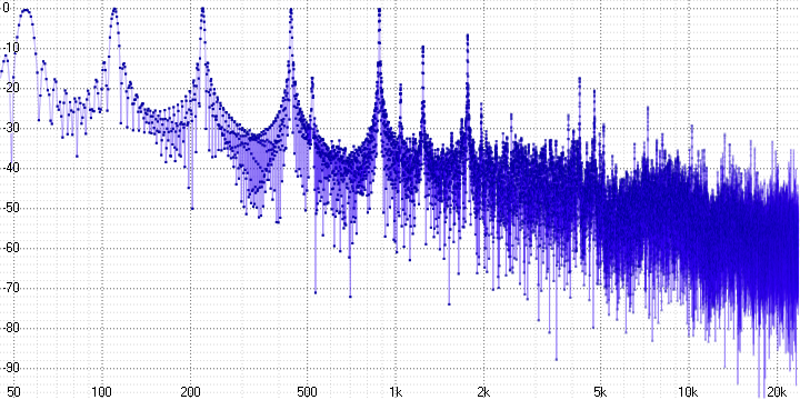
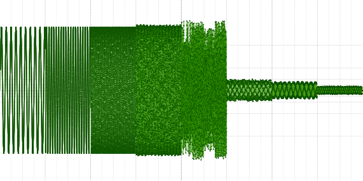
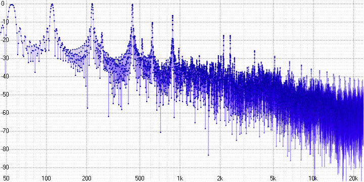
8 tone sequence
Contains notes “la” from controcade (55 Hz) to “la” of the fifth octave (7040 Hz).
Source signal:
Measurement results:
sample length = 4:
sample length = 8:
sample length = 16:
sample length = 32:
Here we can already unequivocally state the presence of pronounced harmonic distortion. Since a sinusoid is a pure tone, any distortion of it leads to the appearance of harmonics - they are clearly visible (at a frequency of 5 kHz in the first graph, for example).
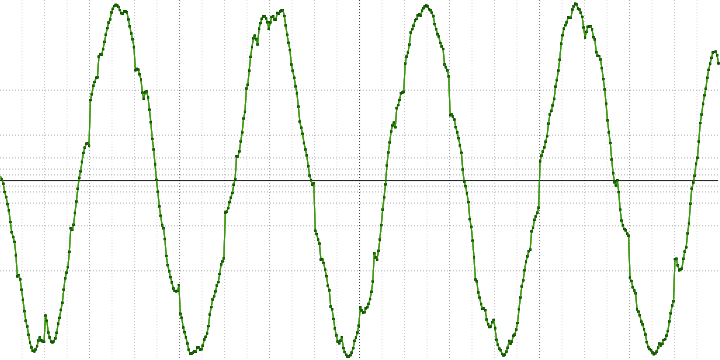
Consider a sine wave with a frequency of 440 Hz from the last measurement a little closer:
Here you can see that it is assembled from pieces from other sinusoids. Also clearly visible and tears at the edges of the blocks.
Testing "acceleration" and dynamic range expansion
In the decoder it is possible to increase the sampling rate by 2 or 4 times and the quantization depth up to 24 bits. Let's test this possibility on the previous signal (with the parameter sample length = 4):
The shape of the signal shows that it has undergone even greater distortion. By frequency response it can be seen that the extended frequency range is filled with noise. Nothing like an expansion of the dynamic range is also observed (for example, in the form of noise reduction).
Conclusion
Of course, from the above graphs it does not at all follow that this codec cannot be used in practice. It is possible that for someone the words “Fractal Compression” and “Chaos Theory” will have much more weight than some kind of graphics. It is equally possible that someone will perceive his distortions as special and pleasant to the ear, which only improve the sound.
But to me personally, the idea of fractal compression as such seems to be far-fetched since the beginning of its appearance and seems to be a kind of “Holy Grail”. Indeed, since the release of the Fractal Geometry of Nature, nothing particularly new has appeared - the same fractal leaves and trees, the Maldebrot and Julia sets, the Koch, Hilbert, Peano curves and the Sierpinski triangles (and the original article did not become an exception in this regard). Moreover, they all have an exclusively geometric nature - no one has yet declared the existence of “audio fractals” endowed with the properties of self-similar sets with fractional metric dimension.
Source: https://habr.com/ru/post/310872/
All Articles