Screen Space Ambient Occlusion
Further, it will be discussed how to implement the Screen Space Ambient Occlusion method for calculating diffused lighting in the C ++ programming language using the API DirectX11.
Consider the formula for calculating the color of a pixel on the screen when using, for example, a parallel light source:
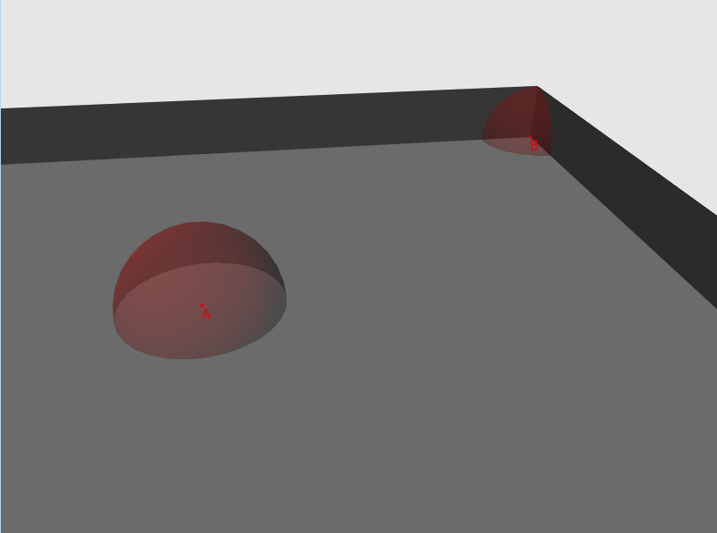
Fig.1 - a drawing with a room and two points, the “visibility” of each point is depicted as a sphere
So, for each vertex in random directions, we add rays and find their intersection with the geometry of the scene. Next, we calculate the length of the resulting line (if the intersection was not found, we will assume that the beam has a certain maximum length for the given scene) and compare it with the threshold value. If the length exceeds the threshold value - then the beam passes the “visibility” test. The number of tests passed divided by the number of rays launched will be the “visibility” factor.
')
Obviously, the high computational complexity of the algorithm makes it inapplicable in real time or for scenes with high dynamics of objects. Also, the effectiveness of the method strongly depends on the polygonal complexity of the scene. This approach is reasonable to use when it is possible to calculate in advance the "visibility" and save it as part of the vertices or in the texture.
Fortunately, the guys at CryTeck (at least I heard that they were the first) came up with a way to calculate the coefficient in real time. It is called Screen Space Ambient Occlusion.
The algorithm of my implementation is as follows:
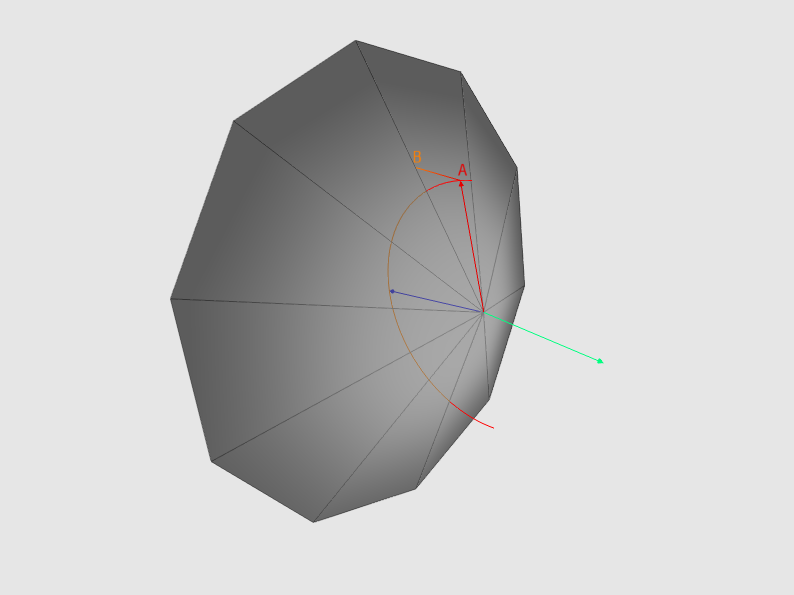
Fig.2 - in blue is depicted the normal vector, in red is the vector obtained in step 3-a. A light green vector is the direction of the Z axis. If the depth value at point A is greater than at point B, this is an overlap. For clarity, the figure uses an orthogonal projection (therefore, the AB line is a straight line)
By applying this algorithm in a pixel shader, we can get the visibility data if we write the rendering result to a texture. The data from this texture can be further used when calculating the illumination of the scene.
So, let's begin.
In order to get screen coordinates from three-dimensional coordinates, we need to perform a series of matrix transformations.
In the general form of such transformations, there are three:
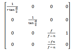
Items 1 and 2 are not important for us, so we proceed immediately to p.3. Let's look at the projection matrix:
After multiplying by this matrix, the coordinates from the camera space go to the projection space

This is followed by a homogeneous division, as a result of this we move to the space NDC

Now let's see how to do the inverse transform. Obviously, we first need pixel coordinates in the shader. I think it is most convenient to use a square covering the entire screen area in NDC space with texture coordinates from (0,0) to (1,1). Here is the vertex data:
You also need to set the point interpolation of the texture data, for example D3D11_FILTER_MIN_MAG_MIP_POINT. By drawing this square, we can either "forward" the vertex data to the pixel shader like this:
Or, directly in the pixel shader, convert the interpolated texture coordinates into the NDC space like this (for more details on this conversion, see Chapter 3):
The coordinates of the pixel in the NDC space we have - now we need to go to the view space. Based on the properties of matrices:

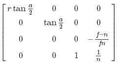
For our purposes, we must have an inverse projection matrix. She looks like this:
But it is not enough for us to simply multiply the two-dimensional point in it in the NDC space and make a uniform division - we also need to have data on the depth of the point that we transform. I want to use depth in the form of space - let's do some algebraic transformations and find out if this is possible. First, we express the transition of a point from the species to the NDC space:
Now, we multiply by the inverse projection matrix:

Then, simplify X and Y and expand the brackets in W:
Further we will continue simplification in W:
And the final touch - cut 1 / n:

It turns out that after multiplying by the inverse matrix of the projection, we need to multiply the result by the depth in the view space. So we proceed. First, prepare the data in the NDC space in the vertex shader:
Then we will do the main work in the pixel shader:
We have coordinates in space of the form. Go ahead.
2.1 Offset data
So, we have the coordinates of the pixel being processed in the view space. Further from the point with these coordinates, we need to send N rays in random directions. Unfortunately, the HLSL API does not have a tool with which we could get a random or pseudo-random value during the execution of a shader regardless of external data (well, or I just don’t know about the existence of such technologies) - therefore, we will prepare such data in advance. In order to get them in a shader, the easiest way is to use a texture. Obviously, its “weight” and the limit of data values depend on the pixel format. For our purposes, the DXGI_FORMAT_R8G8B8A8_UNORM format is quite suitable. Now let's deal with the size. Probably the easiest, descriptive and at the same time non-optimal way is to create a texture with a length and width equal to the screen resolution. In this case, we simply select the data by the value of the texture coordinates of the square, which, recall, are in the range of (0,0) to (1,1). But what will happen if we go beyond these limits? Then the rules specified in the D3D11_TEXTURE_ADDRESS_MODE enumeration come into play. In this case, we are interested in the value of D3D11_TEXTURE_ADDRESS_MIRROR. The result of this addressing rule is shown in Figure 3.

Figure 3 - an example of using D3D11_TEXTURE_ADDRESS_MIRROR "
If we use this approach, then for our purposes, differences will be acceptable (see Figure 4).
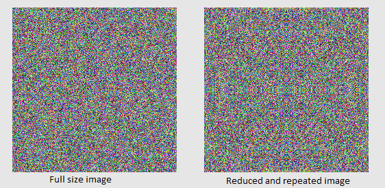
Fig.4 - primitive with texture overlay 256x256 and with coordinates from 0 to 1 and primitive with texture overlay 4x4 with coordinates from 0 to 64 and addressing D3D11_TEXTURE_ADDRESS_MIRROR
Now, finally, let's fill the texture with data. In the shader, we will form a random direction vector from the R, G, and B texel components, so we do not use the alpha channel (you can consider it as a component of W, which is zero for vectors in a homogeneous space). As a result, the code is something like this:
I also want to draw attention to the fact that the smaller the texture size, the clearer the image will be (see Figure 5):
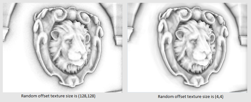
Fig.5 - a demonstration of the difference between textures of 128x128 and 4x4 offsets
Well, our texture is ready - it remains only to get this data in the shader. But we remember that we have texture coordinates from 0 to 1, and we need to use coordinates from 0 to N, where N> 0. This problem is solved very simply at the stage of preparing the shader - you need to know how much you need to multiply the length and How much you need to multiply the width of the texture so that it takes up the entire screen. Suppose that the screen resolution is 1024x768, and the size of the texture is 2x4, then we get:
Now we will express the coefficients:
As a result, we get the following code:
Perhaps, in your case, it will be more rational to store these coordinates of the sample from the displacement texture as vertex data, thereby obtaining a ready-made interpolation value.
Further, since we chose the DXGI_FORMAT_R8G8B8A8_UNORM format, our offset is in the space from 0 to 1. Transfer it to the space (-1, 1) (for a detailed description of the transformation, see Chapter 3):
Now we have a displacement vector!
2.2 The core of the displacement vectors
One vector is nice, but we need to start up N vectors. We can get a certain factor of the displacement of texture coordinates ranging from 0 to N and do something like this:
This option is too resource intensive. Let's try to get an acceptable result using only one sample from the texture. Our goal is to achieve a relatively heterogeneous distribution of vectors both within the processed pixel and relative to the neighboring ones. Let's take N prearranged random vectors and each of them is applicable to our displacement vector with a specific mathematical operation. This set is called the "Core of the displacement vectors". I assure you, it's easier than I described)
Prepare our core:
Values for each component are generated from -1 to 1. Please note that vectors are not of unit length. This is important because it significantly affects the final image. In fig. 6 that the vectors of non-unit length, when projected, form a more concentrated set of points.

Fig.6 - projection of vectors of non-unit length forms a more concentrated set of points. For greater clarity, orthogonal projection is used.
Well, the kernel is ready - it remains to use it in the shader. As a mathematical operation, I decided to use "Reflection of the vector." This tool is very useful and widely used - for example, if we need to get the reflected vector to the light source when calculating the specular lighting or if we need to know which way the ball will fly, bounced off the wall. The formula for calculating the reflected vector is as follows:

where v is the vector that we are going to reflect, n is the normal to the surface, relative to which we will reflect the vector (see fig.7)

Fig.7 - visualization of the formula of the reflected vector
The last thing we need to do with the vector is to ensure that it is within the normal-oriented hemisphere. To do this, we will change its direction if its scalar product with a normal is less than zero. As a result, we got the following code:
Please note that we do not normalize the result of the reflect () operation.
Let's look back and see what happened. So:
Now we have everything we need in order to finally know what is around us. We continue. Multiply our vector by a certain scalar occlusionRadius and add it to the point of our pixel in the view space. It is reasonable to allow the artist to regulate the value of occlusionRadius.
Formally speaking, in the view space we obtained a samplingPosV point, which is located at a distance from our pixel in the direction of samplingRayL. Next, we project the resulting point onto the screen, while not forgetting to produce a “uniform division” in order to take into account the depth:
We are in the NDC space. Now we need to go to the texture coordinate space. To do this, we transform our point from the range of values from -1 to 1 to the area from 0 to 1. Note that the Y axis is directed in the opposite direction. (see figure 8)

Fig.8 - Demonstration of coordinate axes for NDC and texture coordinate space
Let's first convert the X coordinate. In general, one-dimensional transformations of this kind can be performed as follows: first we subtract the minimum value of the range, then divide by the width of the range (maximum minus minimum), then multiply the resulting coefficient by the width of the range of the new space and add to the result minimum value of new space. I assure you it is easier to do than to say. For our case, suppose that Nx is the X coordinate in the NDC space, Tx is the X coordinate in the texture coordinate space. It turns out the following:

Since the Y coordinate in the NDC space is directed in the opposite direction, it is necessary to act somewhat differently. We cannot simply take the value with the opposite sign, since we will immediately go beyond the permissible limits. Hmm ... Imagine a point in the lower right corner of the screen - in the NDC space its coordinates will be (1, -1), and in the coordinate space of the texture - (1, 1). Now imagine a point in the upper left corner - in its NDC space the coordinates will be (-1, 1), and in the coordinate space of the texture - (0, 0). The following pattern emerges: for the boundary regions, Y takes the maximum value in one coordinate system and the minimum in the other and vice versa. Therefore, when we get our coefficient - we will subtract it from the unit.

We can solve this problem in another way. The solution is presented in Appendix 1.
As a result, in the shader we get the following code:
I add that you can combine the transformation to the texture coordinate and projecting in one matrix as follows (P is the projection matrix):

Very little is left! Hurry, hurry! According to the coordinates obtained in the previous paragraph, we make a sample of the texture with the data.
Component w stores depth data - take it and! And ... And what should we do with them !? Let's think about it. We are in the form of space - the Z axis coincides with the direction of the camera. Therefore, the smaller the obtained depth, the closer the object is to us. Let me remind you that we have projected a point, which is located at some distance from our pixel in the view space. The texture also stores depth in view space. What do we learn if we compare the depth of the texture with the depth of our point? If the depth value from the texture is less than the depth of the point, then something is located closer to the camera and our point will not be visible. Accordingly, our point is visible if it is closer to the camera than this “something”. By the way, about also works ShadowMapping. It’s as if you need to make a difficult maneuver by car, and you don’t see what’s going on below and you’re asking a friend to adjust your movement. But he was drunk and thought that it would be very funny to tell you the data opposite to what you expected ... But this is not our case)
So, the fewer points from the N set can be seen by the camera, the less diffuse lighting our pixel receives. You can consider the situation a little differently - let's imagine that we are looking from our pixel in the direction of its normal (because the rays are distributed within the hemisphere oriented by the normal). The fewer points from the N set are visible to the camera, the smaller the number of scene objects we can see from our pixel (because more and more “geometry” of the scene objects blocks our view) - hence the less access to the ambient light of the scene (Damn! Dad made my poster "Iron maiden" with your skis! Pikachu! I challenge you !!)
It should also be noted that a certain object of the scene, the depth of which we received, may be so far that it does not affect access to diffused light to a pixel point (see. Fig. 9)

Fig.9 - The point q, though closer to the camera, is located too far from the pixel point P and cannot affect its illumination.
I suggest not just adding 1, but a certain coefficient depending on the distance:
Notice that we form the distance coefficient based on the depth of the pixel point, and not the point we projected — we used it to see if there is something in front of us, but now we need to understand how far this “something” This is from us. I also added the ability to adjust the intensity through the harshness parameter.
In general, this is the main part of the algorithm, so to say heart of it all. Let's look at the whole cycle of working with displacement vectors:
Let's look at the result!

"Hey! What the heck is that! And where is FarCry?! ”- you ask. "Easy!" - I will answer you. “Chip and Dale rush to the rescue!” Oh, this is not from that article - “Blur hurries to the rescue!”
5.1 is the easiest option.
Blur effect, or Blur, is a very useful tool that is used in many areas of graphics. I would compare it with electrical tape (blue! This is important) - with its help, you can fix or improve something, but you can hardly fix the phone that fell on the tile from the height of the cabinet (although instructions like “Wrap it with insulation, and everything will be fine "Met more than once).
The essence of the effect is simple: for each texel, get the arithmetic average of the colors of its neighbors.
So, suppose we have a texel with coordinates P - let's calculate the arithmetic average of the colors of its neighbors in R (AreaWidth by AreaHeight pixels). Something like this (I deliberately do not check for exceeding the array bounds. About this below):
5.2 Gauss filter
Now let's do the following: we will multiply the color of each neighbor by the value from the matrix whose dimension is equal to AreaWidth by AreaHeight. We will also ensure that the sum of all elements of the matrix is equal to 1 - this will save us from having to divide by the size of the region, because now it will be a special case of the arithmetic average weighted. Such a matrix is formally called the “Convolution Matrix”, also called the “Core”, and its elements are called “weights”. Why do you need it?So we have more opportunities - by controlling the value of the scales, we can achieve, for example, the effect of pulsation or gradual blurring. There is also a whole family of filters based on the convolution matrix — a clarity enhancement filter, a median filter, erosion filters, and a build-up.
The most common filter for blurring is a Gaussian filter. Its important property is linear separability - This allows us to first blur the input image in rows, then the image blurred in rows to blur in columns, performing one cycle with the values of a one-dimensional filter, the formula of which looks like:

where x is an integer from -AreaWidth / 2 to AreaWidth / 2, q is the so-called "Standard deviation of the Gaussian distribution" (the standard deviation of the Gaussian distribution)
I implemented the function that forms the filter matrix:
I use a radius of 5, and the deviation is 5 squared.
5.3 Shader and everything connected with it.
We will use two textures - one with the original data, the other for storing the intermediate result. Create both textures with dimensions corresponding to the screen resolution and pixel format DXGI_FORMAT_R32G32B32A32_FLOAT. You can, of course, not having lost much in quality, reduce the size of the textures, but in this case I decided not to. We will work with textures according to the following scheme:
As before, we will work with a square in the NDC space, which occupies the entire screen area, with texture coordinates from 0 to 1. Now is the time to think about how to handle the output beyond the texture boundaries.
Implementing checks directly in the shader code is too resource intensive. Let's see what options we have if we still go beyond the boundaries of the area. As I said earlier, in this case, the rules specified in the D3D11_TEXTURE_ADDRESS_MODE enumeration come into play. The D3D11_TEXTURE_ADDRESS_CLAMP rule is appropriate. The following happens: each of the coordinates is limited to the range [0, 1]. That is, if we do a sample with coordinates (1.1, 0), we get the data of the texel with coordinates (1, 0), if we choose (-0.1, 0) for the coordinates, we get the data in (0, 0). The same for Y (see fig. 12).

Fig.12 demonstration of D3D11_TEXTURE_ADDRESS_CLAMP with regard to the size of the filter
The last thing left to know is how much we need to move in order to move one pixel in the texture coordinate space. This problem is solved simply - suppose that the screen resolution is 1024 by 768 pixels, then, for example, the center of the screen in space from 0 to 1 will be (512/1024, 384/768) = (0.5 0.5), and the point located by one pixel from the upper left corner - (1/1024, 1/768). You can also express the solution of this problem in the form of an equation. Let (Sx, Sy) be our starting position, (Ex, Ey) be the ending position, then the answer to the question “To which part of the screen do we need to move in order to move from S to E?” Will look like this:

Suppose we want to move one pixel from the top left corner of the screen, then the equation will look like this:

Express for F and get:

Now, perhaps, we can give the pixel shader code:
The vertex shader did not give here, because nothing special happens there - just “forward” the data further. Let's see what we did:

Fig.13 demonstration of blur without facets
Not bad, but now we need to solve the problem of blurry edges. In our case, to make it easier than it might seem at first glance - after all, we already have all the necessary data! If we are in screen space, then it is enough for us to track the abrupt changes in the data of the normal and depth. If the scalar product of the normals or the absolute value of the difference between the depths of the neighboring and processed pixel is more or less than certain values, then we assume that the pixel being processed belongs to the line of the face. I wrote a small shader that highlights the faces in yellow. The principle of operation is the same as for blurring - we pass first vertically, then horizontally. We will compare the two neighbors either to the left and to the right, or at the top and bottom, depending on the direction. It turned out like this:

Figure 14 Demonstrating facet selection.
How do we use this when blurring? Very simple!We will not take into account the color of those neighbors that are very far away or significantly differ in the direction of the normals from the pixel, the color of which we consider. Only now it is necessary to divide the result by the amount of weights processed. Here is the code:
The result was this:

When I was finishing work on this article, as a result of another test, I found out that the result of the overlap is unstable with respect to the camera direction. In order to fix this, we need to translate the coordinates of the pixel being processed and the points from clause 3 from the view space to the world one. In my case, the problem is aggravated by the fact that all the important data I store in the space of the form, so in a cycle over all the rays we need to convert either the depth of the point into the space of the form, or the depth from the tekstrura into the world space. We also need to remember to transfer the normal to the world space, but not so critical, since it does not depend on the cycle.
I want to thank the reader for the attention to my article, and I hope that the information contained in it was accessible, interesting and useful. I would also like to thank Leonid ForhaxeD for his article - I took a lot from it and tried to improve it.
The source code of the sample can be downloaded at github.com/AlexWIN32/SSAODemo . Suggestions and comments regarding the work of the example as a whole or its individual subsystems can be sent to me by mail or leave as comments. I wish you success!
Consider the formula for calculating the color of a pixel on the screen when using, for example, a parallel light source:
LitColor = Ambient + Diffuse + SpecularOr, more formally, the sum of diffused, absorbed and specular illuminations. Each of them is calculated as follows:
(material color) * (source color) * (intensity coefficient)For a long time in applications of interactive graphics, the coefficient of the intensity of diffused (ambient) lighting was constant, but now we can calculate it in real time. I would like to talk about one of these methods - ambient occlusion, or rather its optimization - screen space ambient occlusion. Let's talk first about the ambient occlusion method. Its essence is as follows - for each top of the scene to form a factor that will determine the degree of "visibility" of the rest of the scene.
Fig.1 - a drawing with a room and two points, the “visibility” of each point is depicted as a sphere
So, for each vertex in random directions, we add rays and find their intersection with the geometry of the scene. Next, we calculate the length of the resulting line (if the intersection was not found, we will assume that the beam has a certain maximum length for the given scene) and compare it with the threshold value. If the length exceeds the threshold value - then the beam passes the “visibility” test. The number of tests passed divided by the number of rays launched will be the “visibility” factor.
')
Obviously, the high computational complexity of the algorithm makes it inapplicable in real time or for scenes with high dynamics of objects. Also, the effectiveness of the method strongly depends on the polygonal complexity of the scene. This approach is reasonable to use when it is possible to calculate in advance the "visibility" and save it as part of the vertices or in the texture.
Fortunately, the guys at CryTeck (at least I heard that they were the first) came up with a way to calculate the coefficient in real time. It is called Screen Space Ambient Occlusion.
The algorithm of my implementation is as follows:
- 1. Take NDC (normalized device coordinates) or pixel texture coordinates and convert them to a point in the camera space, using the depth data;
- 2. From this point in the random directions we let N rays;
- 3. For each of the N rays:
- 3-a. multiply (scale) our ray (vector) by a certain number (scalar) and add it to the point from item 1;
- 3-b. Transform the resulting point into NDC space, and then into texture coordinates;
- 3-c. From the texture, we get the depth value for this point;
- 3rd. If the resulting value is less than the depth of the point obtained in paragraph 3-a, then there is an “overlap” (see Fig. 2). It is necessary to take into account that these values belong to the same coordinate system;
- 3-f. We obtain the “overlap” factor based on the dependence “The farther a point from p. 3 is on the point from p. 1, the less potential overlap from this point”. Accumulate its value.
- 4. We obtain the general factor of “overlap”, which is equal to the total total overlap of the / N rays. Since the common factor belongs to [0,1], and visibility is inversely proportional to the overlap, then it is equal to 1 - overlap.
Fig.2 - in blue is depicted the normal vector, in red is the vector obtained in step 3-a. A light green vector is the direction of the Z axis. If the depth value at point A is greater than at point B, this is an overlap. For clarity, the figure uses an orthogonal projection (therefore, the AB line is a straight line)
By applying this algorithm in a pixel shader, we can get the visibility data if we write the rendering result to a texture. The data from this texture can be further used when calculating the illumination of the scene.
So, let's begin.
1. Conversion
In order to get screen coordinates from three-dimensional coordinates, we need to perform a series of matrix transformations.
In the general form of such transformations, there are three:
- 1. From local coordinates to world ones - transfer all objects to a common coordinate system
- 2. From world coordinates to view coordinates - to orient all objects relative to the “camera”
- 3. From view coordinates to projection coordinates - project the vertices of the objects on the plane. We use the perspective projection, which implies the so-called homogeneous divide - the division of the components x and at the apex by its depth - the component z.
Items 1 and 2 are not important for us, so we proceed immediately to p.3. Let's look at the projection matrix:
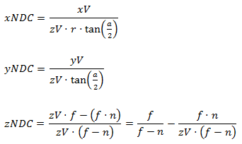
After multiplying by this matrix, the coordinates from the camera space go to the projection space
This is followed by a homogeneous division, as a result of this we move to the space NDC
Now let's see how to do the inverse transform. Obviously, we first need pixel coordinates in the shader. I think it is most convenient to use a square covering the entire screen area in NDC space with texture coordinates from (0,0) to (1,1). Here is the vertex data:
struct ScreenQuadVertex { D3DXVECTOR3 pos = {0.0f, 0.0f, 0.0f}; D3DXVECTOR2 tc = {0.0f, 0.0f}; ScreenQuadVertex(){} ScreenQuadVertex(const D3DXVECTOR3 &Pos, const D3DXVECTOR2 &Tc) : pos(Pos), tc(Tc){} }; std::vector<ScreenQuadVertex> vertices = { {{-1.0f, -1.0f, 0.0f}, {0.0f, 1.0f}}, {{-1.0f, 1.0f, 0.0f}, {0.0f, 0.0f}}, {{ 1.0f, 1.0f, 0.0f}, {1.0f, 0.0f}}, {{ 1.0f, -1.0f, 0.0f}, {1.0f, 1.0f}}, }; You also need to set the point interpolation of the texture data, for example D3D11_FILTER_MIN_MAG_MIP_POINT. By drawing this square, we can either "forward" the vertex data to the pixel shader like this:
VOut output; output.posN = float4(input.posN, 1.0f); output.tex = input.tex; output.eyeRayN = float4(output.posN.xy, 1.0f, 1.0f); Or, directly in the pixel shader, convert the interpolated texture coordinates into the NDC space like this (for more details on this conversion, see Chapter 3):
float4 posN; posN.x = (Input.tex.x * 2.0f) - 1.0f; posN.y = (Input.tex.y * -2.0f) + 1.0f; The coordinates of the pixel in the NDC space we have - now we need to go to the view space. Based on the properties of matrices:
For our purposes, we must have an inverse projection matrix. She looks like this:
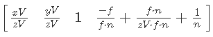
But it is not enough for us to simply multiply the two-dimensional point in it in the NDC space and make a uniform division - we also need to have data on the depth of the point that we transform. I want to use depth in the form of space - let's do some algebraic transformations and find out if this is possible. First, we express the transition of a point from the species to the NDC space:
Now, we multiply by the inverse projection matrix:
Then, simplify X and Y and expand the brackets in W:
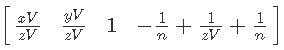
Further we will continue simplification in W:
And the final touch - cut 1 / n:
It turns out that after multiplying by the inverse matrix of the projection, we need to multiply the result by the depth in the view space. So we proceed. First, prepare the data in the NDC space in the vertex shader:
output.eyeRayN = float4(output.posN.xy, 1.0f, 1.0f); Then we will do the main work in the pixel shader:
float4 normalDepthData = normalDepthTex.Sample(normalDepthSampler, input.tex); float3 viewRay = mul(input.eyeRayN, invProj).xyz; viewRay *= normalDepthData.w; We have coordinates in space of the form. Go ahead.
2. Ray tracing
2.1 Offset data
So, we have the coordinates of the pixel being processed in the view space. Further from the point with these coordinates, we need to send N rays in random directions. Unfortunately, the HLSL API does not have a tool with which we could get a random or pseudo-random value during the execution of a shader regardless of external data (well, or I just don’t know about the existence of such technologies) - therefore, we will prepare such data in advance. In order to get them in a shader, the easiest way is to use a texture. Obviously, its “weight” and the limit of data values depend on the pixel format. For our purposes, the DXGI_FORMAT_R8G8B8A8_UNORM format is quite suitable. Now let's deal with the size. Probably the easiest, descriptive and at the same time non-optimal way is to create a texture with a length and width equal to the screen resolution. In this case, we simply select the data by the value of the texture coordinates of the square, which, recall, are in the range of (0,0) to (1,1). But what will happen if we go beyond these limits? Then the rules specified in the D3D11_TEXTURE_ADDRESS_MODE enumeration come into play. In this case, we are interested in the value of D3D11_TEXTURE_ADDRESS_MIRROR. The result of this addressing rule is shown in Figure 3.
Figure 3 - an example of using D3D11_TEXTURE_ADDRESS_MIRROR "
If we use this approach, then for our purposes, differences will be acceptable (see Figure 4).
Fig.4 - primitive with texture overlay 256x256 and with coordinates from 0 to 1 and primitive with texture overlay 4x4 with coordinates from 0 to 64 and addressing D3D11_TEXTURE_ADDRESS_MIRROR
Now, finally, let's fill the texture with data. In the shader, we will form a random direction vector from the R, G, and B texel components, so we do not use the alpha channel (you can consider it as a component of W, which is zero for vectors in a homogeneous space). As a result, the code is something like this:
for(int y = 0; y < texHeight; y++){ for(int x = 0; x < texWidth; x++){ char* channels = reinterpret_cast<char*>(&data[y * texWidth + x]); channels[0] = rand() % 255; //r channels[1] = rand() % 255; //g channels[2] = rand() % 255; //b channels[3] = 0; //a } } I also want to draw attention to the fact that the smaller the texture size, the clearer the image will be (see Figure 5):
Fig.5 - a demonstration of the difference between textures of 128x128 and 4x4 offsets
Well, our texture is ready - it remains only to get this data in the shader. But we remember that we have texture coordinates from 0 to 1, and we need to use coordinates from 0 to N, where N> 0. This problem is solved very simply at the stage of preparing the shader - you need to know how much you need to multiply the length and How much you need to multiply the width of the texture so that it takes up the entire screen. Suppose that the screen resolution is 1024x768, and the size of the texture is 2x4, then we get:
Now we will express the coefficients:
As a result, we get the following code:
float2 rndTexFactor(fWidth, fHeight); float3 rndData = tex.Sample(randomOffsetsSampler, input.tex * rndTexFactor).rgb; Perhaps, in your case, it will be more rational to store these coordinates of the sample from the displacement texture as vertex data, thereby obtaining a ready-made interpolation value.
Further, since we chose the DXGI_FORMAT_R8G8B8A8_UNORM format, our offset is in the space from 0 to 1. Transfer it to the space (-1, 1) (for a detailed description of the transformation, see Chapter 3):
rndData = normalize(2.0f * rndData - 1.0f); Now we have a displacement vector!
2.2 The core of the displacement vectors
One vector is nice, but we need to start up N vectors. We can get a certain factor of the displacement of texture coordinates ranging from 0 to N and do something like this:
for(int i = 0; i < N; i++){ float3 rndData = tex.Sample(randomOffsetsSampler, input.tex * rndTexFactor + Offset * i).rgb; rndData = normalize(2.0f * rndData - 1.0f); /*...*/ } This option is too resource intensive. Let's try to get an acceptable result using only one sample from the texture. Our goal is to achieve a relatively heterogeneous distribution of vectors both within the processed pixel and relative to the neighboring ones. Let's take N prearranged random vectors and each of them is applicable to our displacement vector with a specific mathematical operation. This set is called the "Core of the displacement vectors". I assure you, it's easier than I described)
Prepare our core:
std::vector<D3DXVECTOR4> kernel(KernelSize); int i = 0; for(D3DXVECTOR4 &k : kernel){ kx = Math::RandSNorm(); ky = Math::RandSNorm(); kz = Math::RandSNorm(); kw = 0.0f; D3DXVec4Normalize(&k, &k); FLOAT factor = (float)i / KernelSize; k *= Math::Lerp(0.1f, 0.9f, factor); i++; } Values for each component are generated from -1 to 1. Please note that vectors are not of unit length. This is important because it significantly affects the final image. In fig. 6 that the vectors of non-unit length, when projected, form a more concentrated set of points.
Fig.6 - projection of vectors of non-unit length forms a more concentrated set of points. For greater clarity, orthogonal projection is used.
Well, the kernel is ready - it remains to use it in the shader. As a mathematical operation, I decided to use "Reflection of the vector." This tool is very useful and widely used - for example, if we need to get the reflected vector to the light source when calculating the specular lighting or if we need to know which way the ball will fly, bounced off the wall. The formula for calculating the reflected vector is as follows:
where v is the vector that we are going to reflect, n is the normal to the surface, relative to which we will reflect the vector (see fig.7)
Fig.7 - visualization of the formula of the reflected vector
The last thing we need to do with the vector is to ensure that it is within the normal-oriented hemisphere. To do this, we will change its direction if its scalar product with a normal is less than zero. As a result, we got the following code:
//float3 kernel[N] - //normalV - float3 rndData = tex.Sample(randomOffsetsSampler, input.tex * rndTexFactor + Offset * i).rgb; rndData = normalize(2.0f * rndData - 1.0f); for(int i = 0; i < N; i++){ float3 samplingRayL = reflect(kernel[N], rndData); samplingRayL *= sign(dot(samplingRayL, normalV)); /*...*/ } Please note that we do not normalize the result of the reflect () operation.
3. From ray to spot on screen
Let's look back and see what happened. So:
- Using the depth data, we obtained the pixel coordinates in the view space.
- We got N rays randomly distributed relative to each other.
Now we have everything we need in order to finally know what is around us. We continue. Multiply our vector by a certain scalar occlusionRadius and add it to the point of our pixel in the view space. It is reasonable to allow the artist to regulate the value of occlusionRadius.
//viewRay - float3 samplingPosV = viewRay + (samplingRayL * occlusionRadius); Formally speaking, in the view space we obtained a samplingPosV point, which is located at a distance from our pixel in the direction of samplingRayL. Next, we project the resulting point onto the screen, while not forgetting to produce a “uniform division” in order to take into account the depth:
float4 samplingPosH = mul(float4(samplingPosV, 1.0f), proj); float2 samplingRayN = samplingRayH.xy / samplingRayH.w; We are in the NDC space. Now we need to go to the texture coordinate space. To do this, we transform our point from the range of values from -1 to 1 to the area from 0 to 1. Note that the Y axis is directed in the opposite direction. (see figure 8)
Fig.8 - Demonstration of coordinate axes for NDC and texture coordinate space
Let's first convert the X coordinate. In general, one-dimensional transformations of this kind can be performed as follows: first we subtract the minimum value of the range, then divide by the width of the range (maximum minus minimum), then multiply the resulting coefficient by the width of the range of the new space and add to the result minimum value of new space. I assure you it is easier to do than to say. For our case, suppose that Nx is the X coordinate in the NDC space, Tx is the X coordinate in the texture coordinate space. It turns out the following:
Since the Y coordinate in the NDC space is directed in the opposite direction, it is necessary to act somewhat differently. We cannot simply take the value with the opposite sign, since we will immediately go beyond the permissible limits. Hmm ... Imagine a point in the lower right corner of the screen - in the NDC space its coordinates will be (1, -1), and in the coordinate space of the texture - (1, 1). Now imagine a point in the upper left corner - in its NDC space the coordinates will be (-1, 1), and in the coordinate space of the texture - (0, 0). The following pattern emerges: for the boundary regions, Y takes the maximum value in one coordinate system and the minimum in the other and vice versa. Therefore, when we get our coefficient - we will subtract it from the unit.
We can solve this problem in another way. The solution is presented in Appendix 1.
As a result, in the shader we get the following code:
float2 samplingTc; samplingTc.x = 0.5f * samplingRayN.x + 0.5f; samplingTc.y = -0.5f * samplingRayN.y + 0.5f; I add that you can combine the transformation to the texture coordinate and projecting in one matrix as follows (P is the projection matrix):
4. Work with depth data
Very little is left! Hurry, hurry! According to the coordinates obtained in the previous paragraph, we make a sample of the texture with the data.
float sampledDepth = normalDepthTex.Sample(normalDepthSampler, samplingTc).w; Component w stores depth data - take it and! And ... And what should we do with them !? Let's think about it. We are in the form of space - the Z axis coincides with the direction of the camera. Therefore, the smaller the obtained depth, the closer the object is to us. Let me remind you that we have projected a point, which is located at some distance from our pixel in the view space. The texture also stores depth in view space. What do we learn if we compare the depth of the texture with the depth of our point? If the depth value from the texture is less than the depth of the point, then something is located closer to the camera and our point will not be visible. Accordingly, our point is visible if it is closer to the camera than this “something”. By the way, about also works ShadowMapping. It’s as if you need to make a difficult maneuver by car, and you don’t see what’s going on below and you’re asking a friend to adjust your movement. But he was drunk and thought that it would be very funny to tell you the data opposite to what you expected ... But this is not our case)
So, the fewer points from the N set can be seen by the camera, the less diffuse lighting our pixel receives. You can consider the situation a little differently - let's imagine that we are looking from our pixel in the direction of its normal (because the rays are distributed within the hemisphere oriented by the normal). The fewer points from the N set are visible to the camera, the smaller the number of scene objects we can see from our pixel (because more and more “geometry” of the scene objects blocks our view) - hence the less access to the ambient light of the scene (Damn! Dad made my poster "Iron maiden" with your skis! Pikachu! I challenge you !!)
It should also be noted that a certain object of the scene, the depth of which we received, may be so far that it does not affect access to diffused light to a pixel point (see. Fig. 9)
Fig.9 - The point q, though closer to the camera, is located too far from the pixel point P and cannot affect its illumination.
I suggest not just adding 1, but a certain coefficient depending on the distance:
float distanceFactor = (1.0f - saturate(abs(viewRay.z - sampledDepth) / occlusionRadius)) * harshness; Notice that we form the distance coefficient based on the depth of the pixel point, and not the point we projected — we used it to see if there is something in front of us, but now we need to understand how far this “something” This is from us. I also added the ability to adjust the intensity through the harshness parameter.
In general, this is the main part of the algorithm, so to say heart of it all. Let's look at the whole cycle of working with displacement vectors:
//viewRay - //normalV - //float3 kernel[N] - //offset - , float totalOcclusion = 0.0f; [unroll] for(int i = 0; i < 16; i++){ float3 samplingRayL = reflect(kernel[i].xyz, offset); samplingRayL *= sign(dot(samplingRayL, normalV)); float3 samplingPosV = viewRay + (samplingRayL * occlusionRadius); float4 samplingPosH = mul(float4(samplingPosV, 1.0f), proj); samplingPosH.xy /= samplingPosH.w; float2 samplingTc; samplingTc.x = 0.5f * samplingPosH.x + 0.5f; samplingTc.y = -0.5f * samplingPosH.y + 0.5f; float sampledDepth = normalDepthTex.Sample(normalDepthSampler, samplingTc).w; if(sampledDepth < samplingPosV.z){ float distanceFactor = (1.0f - saturate(abs(viewRay.z - sampledDepth) / occlusionRadius)); totalOcclusion += distanceFactor * harshness; } } Let's look at the result!
"Hey! What the heck is that! And where is FarCry?! ”- you ask. "Easy!" - I will answer you. “Chip and Dale rush to the rescue!” Oh, this is not from that article - “Blur hurries to the rescue!”
5. Use Blur
5.1 is the easiest option.
Blur effect, or Blur, is a very useful tool that is used in many areas of graphics. I would compare it with electrical tape (blue! This is important) - with its help, you can fix or improve something, but you can hardly fix the phone that fell on the tile from the height of the cabinet (although instructions like “Wrap it with insulation, and everything will be fine "Met more than once).
The essence of the effect is simple: for each texel, get the arithmetic average of the colors of its neighbors.
So, suppose we have a texel with coordinates P - let's calculate the arithmetic average of the colors of its neighbors in R (AreaWidth by AreaHeight pixels). Something like this (I deliberately do not check for exceeding the array bounds. About this below):
D3DXCOLOR **imgData = ...; // D3DXCOLOR avgColor(0.0f, 0.0f, 0.0f, 0.0f); for(INT x = Px - AreaWidth / 2; x <= Px - AreaWidth / 2; x++) for(INT y = Py - AreaHeight / 2; y <= Py - AreaHeight / 2; y++) avgColor += imgData[x][y]; avgColor /= AreaWidth * AreaHeight; 5.2 Gauss filter
Now let's do the following: we will multiply the color of each neighbor by the value from the matrix whose dimension is equal to AreaWidth by AreaHeight. We will also ensure that the sum of all elements of the matrix is equal to 1 - this will save us from having to divide by the size of the region, because now it will be a special case of the arithmetic average weighted. Such a matrix is formally called the “Convolution Matrix”, also called the “Core”, and its elements are called “weights”. Why do you need it?So we have more opportunities - by controlling the value of the scales, we can achieve, for example, the effect of pulsation or gradual blurring. There is also a whole family of filters based on the convolution matrix — a clarity enhancement filter, a median filter, erosion filters, and a build-up.
The most common filter for blurring is a Gaussian filter. Its important property is linear separability - This allows us to first blur the input image in rows, then the image blurred in rows to blur in columns, performing one cycle with the values of a one-dimensional filter, the formula of which looks like:
where x is an integer from -AreaWidth / 2 to AreaWidth / 2, q is the so-called "Standard deviation of the Gaussian distribution" (the standard deviation of the Gaussian distribution)
I implemented the function that forms the filter matrix:
typedef std::vector<float> KernelStorage; KernelStorage GetGaussianKernel(INT Radius, FLOAT Deviation) { float a = (Deviation == -1) ? Radius * Radius : Deviation * Deviation; float f = 1.0f / (sqrtf(2.0f * D3DX_PI * a)); float g = 2.0f * a; KernelStorage outData(Radius * 2 + 1); for(INT x = -Radius; x <= Radius; x++) outData[x + Radius] = f * expf(-(x * x) / a); float summ = std::accumulate(outData.begin(), outData.end(), 0.0f); for(float &w : outData) w /= summ; return outData; } I use a radius of 5, and the deviation is 5 squared.
5.3 Shader and everything connected with it.
We will use two textures - one with the original data, the other for storing the intermediate result. Create both textures with dimensions corresponding to the screen resolution and pixel format DXGI_FORMAT_R32G32B32A32_FLOAT. You can, of course, not having lost much in quality, reduce the size of the textures, but in this case I decided not to. We will work with textures according to the following scheme:
// { // } // { // } As before, we will work with a square in the NDC space, which occupies the entire screen area, with texture coordinates from 0 to 1. Now is the time to think about how to handle the output beyond the texture boundaries.
Implementing checks directly in the shader code is too resource intensive. Let's see what options we have if we still go beyond the boundaries of the area. As I said earlier, in this case, the rules specified in the D3D11_TEXTURE_ADDRESS_MODE enumeration come into play. The D3D11_TEXTURE_ADDRESS_CLAMP rule is appropriate. The following happens: each of the coordinates is limited to the range [0, 1]. That is, if we do a sample with coordinates (1.1, 0), we get the data of the texel with coordinates (1, 0), if we choose (-0.1, 0) for the coordinates, we get the data in (0, 0). The same for Y (see fig. 12).
Fig.12 demonstration of D3D11_TEXTURE_ADDRESS_CLAMP with regard to the size of the filter
The last thing left to know is how much we need to move in order to move one pixel in the texture coordinate space. This problem is solved simply - suppose that the screen resolution is 1024 by 768 pixels, then, for example, the center of the screen in space from 0 to 1 will be (512/1024, 384/768) = (0.5 0.5), and the point located by one pixel from the upper left corner - (1/1024, 1/768). You can also express the solution of this problem in the form of an equation. Let (Sx, Sy) be our starting position, (Ex, Ey) be the ending position, then the answer to the question “To which part of the screen do we need to move in order to move from S to E?” Will look like this:
Suppose we want to move one pixel from the top left corner of the screen, then the equation will look like this:
Express for F and get:
Now, perhaps, we can give the pixel shader code:
cbuffer Data : register(b0) { float4 weights[11]; float2 texFactors; float2 padding; }; cbuffer Data2 : register(b1) { int isVertical; float3 padding2; }; struct PIn { float4 posH : SV_POSITION; float2 tex : TEXCOORD0; }; Texture2D colorTex :register(t0); SamplerState colorSampler :register(s0); float4 ProcessPixel(PIn input) : SV_Target { float2 texOffset = (isVertical) ? float2(texFactors.x, 0.0f) : float2(0.0f, texFactors.y); int halfSize = 5; float4 avgColor = 0; for(int i = -halfSize; i <= halfSize; ++i){ float2 texCoord = input.tex + texOffset * i; avgColor += colorTex.Sample(colorSampler, texCoord) * weights[i + halfSize].x; } return avgColor; } The vertex shader did not give here, because nothing special happens there - just “forward” the data further. Let's see what we did:
Fig.13 demonstration of blur without facets
Not bad, but now we need to solve the problem of blurry edges. In our case, to make it easier than it might seem at first glance - after all, we already have all the necessary data! If we are in screen space, then it is enough for us to track the abrupt changes in the data of the normal and depth. If the scalar product of the normals or the absolute value of the difference between the depths of the neighboring and processed pixel is more or less than certain values, then we assume that the pixel being processed belongs to the line of the face. I wrote a small shader that highlights the faces in yellow. The principle of operation is the same as for blurring - we pass first vertically, then horizontally. We will compare the two neighbors either to the left and to the right, or at the top and bottom, depending on the direction. It turned out like this:
bool CheckNeib(float2 Tc, float DepthV, float3 NormalV) { float4 normalDepth = normalDepthTex.Sample(normalDepthSampler, Tc); float neibDepthV = normalDepth.w; float3 neibNormalV = normalize(normalDepth.xyz); return dot(neibNormalV, NormalV) < 0.8f || abs(neibDepthV - DepthV) > 0.2f; } float4 ProcessPixel(PIn input) : SV_Target { float2 texOffset = (isVertical) ? float2(0.0f, texFactors.y) : float2(texFactors.x, 0.0f); float4 normalDepth = normalDepthTex.Sample(normalDepthSampler, input.tex); float depthV = normalDepth.w; float3 normalV = normalize(normalDepth.xyz); bool onEdge = CheckNeib(input.tex + texOffset, depthV, normalV) || CheckNeib(input.tex - texOffset, depthV, normalV); return onEdge ? float4(1.0f, 1.0f, 0.0f, 1.0f).rgba : colorTex.Sample(colorSampler, input.tex) ; } Figure 14 Demonstrating facet selection.
How do we use this when blurring? Very simple!We will not take into account the color of those neighbors that are very far away or significantly differ in the direction of the normals from the pixel, the color of which we consider. Only now it is necessary to divide the result by the amount of weights processed. Here is the code:
float4 ProcessPixel(PIn input) : SV_Target { float2 texOffset = (isVertical) ? float2(0.0f, texFactors.y) : float2(texFactors.x, 0.0f); float4 normalDepth = normalDepthTex.SampleLevel(normalDepthSampler, input.tex, 0); float depthV = normalDepth.w; float3 normalV = normalize(normalDepth.xyz); int halfSize = 5; float totalWeight = 0.0f; float4 totalColor = 0.0f; [unroll] for(int i = -halfSize; i <= halfSize; ++i){ float2 texCoord = input.tex + texOffset * i; float4 normalDepth2 = normalDepthTex.SampleLevel(normalDepthSampler, texCoord, 0); float neibDepthV = normalDepth2.w; float3 neibNormalV = normalize(normalDepth2.xyz); if(dot(neibNormalV, normalV) < 0.8f || abs(neibDepthV - depthV) > 0.2f) continue; float weight = weights[halfSize + i].x; totalWeight += weight; totalColor += colorTex.Sample(colorSampler, texCoord) * weight; } return totalColor / totalWeight; } The result was this:
6. Unexpected changes
When I was finishing work on this article, as a result of another test, I found out that the result of the overlap is unstable with respect to the camera direction. In order to fix this, we need to translate the coordinates of the pixel being processed and the points from clause 3 from the view space to the world one. In my case, the problem is aggravated by the fact that all the important data I store in the space of the form, so in a cycle over all the rays we need to convert either the depth of the point into the space of the form, or the depth from the tekstrura into the world space. We also need to remember to transfer the normal to the world space, but not so critical, since it does not depend on the cycle.
7. Conclusion
I want to thank the reader for the attention to my article, and I hope that the information contained in it was accessible, interesting and useful. I would also like to thank Leonid ForhaxeD for his article - I took a lot from it and tried to improve it.
The source code of the sample can be downloaded at github.com/AlexWIN32/SSAODemo . Suggestions and comments regarding the work of the example as a whole or its individual subsystems can be sent to me by mail or leave as comments. I wish you success!
Annex 1
:

MinVal — , Range — , Factor — , 0 1. NDC , , , , . NDC

:

:

:

, , , :

:


:

MinVal — , Range — , Factor — , 0 1. NDC , , , , . NDC
:
:
:
, , , :
:
:
Source: https://habr.com/ru/post/310360/
All Articles