ClusterR clustering, part 1
This article focuses on clustering, more precisely, my recently added ClusterR package to CRAN. The details and examples below are mostly based on the Vignette package.
Cluster analysis or clustering is the task of grouping a set of objects so that the objects within one group (called a cluster) are more similar (in one sense or another) to each other than to objects in other groups (clusters). This is one of the main tasks of the research analysis of data and the standard technique of statistical analysis used in various fields, including machine learning, pattern recognition, image analysis, information retrieval, bioinformatics, data compression, computer graphics.
The most well-known examples of clustering algorithms are clustering based on connectivity (hierarchical clustering), clustering based on centers (k-means method, k-medoid method), distribution-based clustering (GMM - Gaussian mixture models) and clustering based on density (DBSCAN - Density-based spatial clustering of applications with noise - spatial clustering of applications with noise based on density, OPTICS - ordering points to identify the clustering structure - ordering points to determine the clustering structure, etc.).
The ClusterR package consists of clustering algorithms based on centers (k-means method, k-means method in mini-groups, k-medoids) and distributions (GMM). The package also offers features for:
')
Gaussian distribution mix is a statistical model for representing normally distributed subpopulations within a general population. The Gaussian mixture of distributions is parameterized by two types of values — a mixture of the weights of the components and the average components or covariances (for the multidimensional case). If the number of components is known, the technique most often used for estimating the parameters of a mixture of distributions is the EM algorithm.
The GMM function in the ClusterR package is an implementation on the R class for modeling data as a Gaussian distribution mixture (GMM) from the Armadillo library with the assumption of diagonal covariance matrices. You can configure the parameters of the function, including gaussian_comps , dist_mode (eucl_dist, maha_dist), seed_mode (static_subset, random_subset, static_spread, random_spread), km_iter, and em_iter (more information about the parameters in the package documentation). I illustrate the GMM function on synthetic data dietary_survey_IBS .
Initially, GMM returns centroids , a covariance matrix (where each row represents a diagonal covariance matrix), weights, and log likelihood functions for each Gaussian component. The predict_GMM function then takes the output of the GMM model and returns possible clusters.
In addition to the already mentioned functions, you can use Optimal_Clusters_GMM to estimate the number of data clusters using either the Akaike information criterion (AIC, Akaike information), or the Bayesian information Bayesian information criterion.
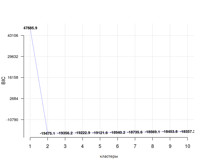
When choosing a model from a predefined set, it is preferable to choose the one with the lowest BIC , here it is true for the number of clusters equal to 2.
Assuming that truth labels are available, you can use the external_validation methods ( rand_index, adjusted_rand_index, jaccard_index, fowlkes_Mallows_index, mirkin_metric, purity, entropy, nmi (normalized mutual information) and var_info (variation of information) to validate output clusters.
And if the parameter summary_stats is set to TRUE, then metrics of specificity, sensitivity, accuracy, completeness, F-measures ( specificity, sensitivity, precision, recall, F-measure, respectively) are also returned.
K-means clustering is a vector quantization method originally used in signal processing that is often used for cluster analysis of data. The goal of k-means clustering is to divide n values into k clusters, in which each value belongs to a cluster with the closest average, which appears as a cluster prototype. This leads to the division of the data area into Voronoi cells. The most commonly used algorithm uses an iterative refinement technique. Due to its widespread usage, it is called the k-means algorithm; in particular, among specialists in the field of computer science, it is also known as the Lloyd's algorithm .
The ClusterR package provides two different k-means functions, KMeans_arma , an R-implementation of the k-means method from the armadillo library, and KMeans_rcpp , which uses the RcppArmadillo package. Both functions lead to the same results, however, they return different signs (the code below illustrates this).
KMeans_arma is faster than the KMeans_rcpp function, however, it initially displays the centroids of only some clusters. Moreover, the number of columns in the data must exceed the number of clusters, otherwise the function will return an error. Clustering will run faster on multi-core machines with OpenMP enabled (for example, -fopenmp in GCC). The algorithm is initialized once, and usually 10 iterations are enough for convergence. The original centroids are distributed using one of the algorithms - keep_existing, static_subset, random_subset, static_spread or random_spread . If seed_mode is equal to keep_existing, the user must pass in the matrix of the centroids.
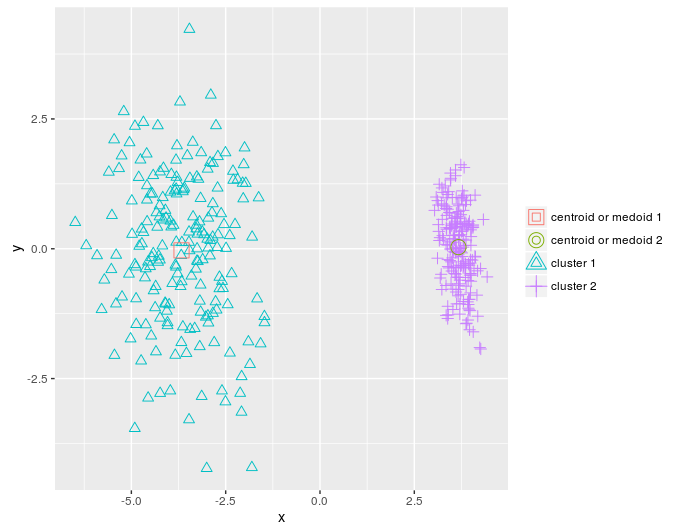
I will reduce the number of measurements in dietary_survey_IBS data using principal component analysis (PCA), namely, the princomp function from the stats package so that you can display a two-dimensional graph of the clusters built as a result.
As stated above, the KMeans_rcpp function offers some additional features compared to the KMeans_arma function:
More details about KMeans_rcpp are in the package documentation. I will illustrate the different parameters of KMeans_rcpp using the example of vector quantization and the OpenImageR package.

The attribute between.SS_DIV_total.SS is (total_SSE - sum (WCSS_per_cluster)) / total_SSE . If there is no pattern in clustering, the intermediate sum of squares will be a very small part of the total sum of squares, and if the attribute between.SS_DIV_total.SS is close to 1.0, the values are clustered well enough.

In addition, you can use the Optimal_Clusters_KMeans feature (which implicitly uses KMeans_rcpp) to determine the optimal number of clusters. The following criteria are available: variance_explained, WCSSE (within-cluster-sum-of-squared-error), dissimilarity, silhouette, distortion_fK, AIC, BIC and Adjusted_Rsquared . The package documentation has more information on each criterion.
The following code example uses the distortion_fK criterion, which is fully described in the article “Selection of K in K-means clustering, Pham., Dimov., Nguyen., (2004)” (“Choice of K in K-means clustering”).
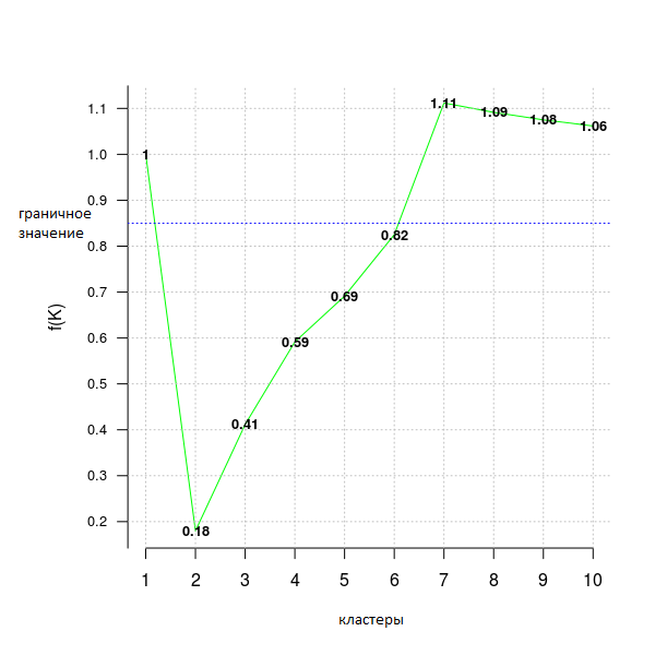
Values less than a fixed limit (here fK_threshold = 0.85) can be recommended for clustering. However, there is more than one optimal partitioning into clusters, so f (K) should be used only to assume their number, but the final decision on whether to accept this value or not is up to the user.
The k-means method in mini-groups is a variation of the classic k-means algorithm. It is especially useful for large data sets, because instead of using the entire set (as in k-means), mini-groups are taken from random data values in order to optimize the objective function.
The parameters of the MiniBatchKmeans algorithm are almost the same as the KMeans_rcpp functions from the ClusterR package. The most important difference is the batch_size parameter (size of mini-groups) and init_fraction (the percentage of data for determining the initial centroids, which is used if the initializer is 'kmeans ++' or 'quantile_init').
I will use the example of vector quantization to show the difference in computation time and quality of the output of the KMeans_rcpp and MiniBatchKmeans functions.

First, perform k-means clustering.

Now k-means clustering in mini-groups .

Despite the slight difference in output quality, k-means in mini-groups returns an average of two times faster than the classic k-means method for this data set.
To implement the k-means method in mini-groups, I used the following resources:
Cluster analysis or clustering is the task of grouping a set of objects so that the objects within one group (called a cluster) are more similar (in one sense or another) to each other than to objects in other groups (clusters). This is one of the main tasks of the research analysis of data and the standard technique of statistical analysis used in various fields, including machine learning, pattern recognition, image analysis, information retrieval, bioinformatics, data compression, computer graphics.
The most well-known examples of clustering algorithms are clustering based on connectivity (hierarchical clustering), clustering based on centers (k-means method, k-medoid method), distribution-based clustering (GMM - Gaussian mixture models) and clustering based on density (DBSCAN - Density-based spatial clustering of applications with noise - spatial clustering of applications with noise based on density, OPTICS - ordering points to identify the clustering structure - ordering points to determine the clustering structure, etc.).
The ClusterR package consists of clustering algorithms based on centers (k-means method, k-means method in mini-groups, k-medoids) and distributions (GMM). The package also offers features for:
')
- validating output with truth labels;
- outputting results on a contour or two-dimensional graph;
- prediction of new observations;
- estimates of the optimal number of clusters for each individual algorithm.
Gaussian mixture of distributions (GMM - Gaussian mixture models)
Gaussian distribution mix is a statistical model for representing normally distributed subpopulations within a general population. The Gaussian mixture of distributions is parameterized by two types of values — a mixture of the weights of the components and the average components or covariances (for the multidimensional case). If the number of components is known, the technique most often used for estimating the parameters of a mixture of distributions is the EM algorithm.
The GMM function in the ClusterR package is an implementation on the R class for modeling data as a Gaussian distribution mixture (GMM) from the Armadillo library with the assumption of diagonal covariance matrices. You can configure the parameters of the function, including gaussian_comps , dist_mode (eucl_dist, maha_dist), seed_mode (static_subset, random_subset, static_spread, random_spread), km_iter, and em_iter (more information about the parameters in the package documentation). I illustrate the GMM function on synthetic data dietary_survey_IBS .
library(ClusterR) data(dietary_survey_IBS) dim(dietary_survey_IBS) ## [1] 400 43 X = dietary_survey_IBS[, -ncol(dietary_survey_IBS)] # ( ) y = dietary_survey_IBS[, ncol(dietary_survey_IBS)] # dat = center_scale(X, mean_center = T, sd_scale = T) # gmm = GMM(dat, 2, dist_mode = "maha_dist", seed_mode = "random_subset", km_iter = 10, em_iter = 10, verbose = F) # , pr = predict_GMM(dat, gmm$centroids, gmm$covariance_matrices, gmm$weights) Initially, GMM returns centroids , a covariance matrix (where each row represents a diagonal covariance matrix), weights, and log likelihood functions for each Gaussian component. The predict_GMM function then takes the output of the GMM model and returns possible clusters.
In addition to the already mentioned functions, you can use Optimal_Clusters_GMM to estimate the number of data clusters using either the Akaike information criterion (AIC, Akaike information), or the Bayesian information Bayesian information criterion.
opt_gmm = Optimal_Clusters_GMM(dat, max_clusters = 10, criterion = "BIC", dist_mode = "maha_dist", seed_mode = "random_subset", km_iter = 10, em_iter = 10, var_floor = 1e-10, plot_data = T) When choosing a model from a predefined set, it is preferable to choose the one with the lowest BIC , here it is true for the number of clusters equal to 2.
Assuming that truth labels are available, you can use the external_validation methods ( rand_index, adjusted_rand_index, jaccard_index, fowlkes_Mallows_index, mirkin_metric, purity, entropy, nmi (normalized mutual information) and var_info (variation of information) to validate output clusters.
res = external_validation(dietary_survey_IBS$class, pr$cluster_labels, method = "adjusted_rand_index", summary_stats = T) res ## ## ---------------------------------------- ## purity : 1 ## entropy : 0 ## normalized mutual information : 1 ## variation of information : 0 ## ---------------------------------------- ## specificity : 1 ## sensitivity : 1 ## precision : 1 ## recall : 1 ## F-measure : 1 ## ---------------------------------------- ## accuracy OR rand-index : 1 ## adjusted-rand-index : 1 ## jaccard-index : 1 ## fowlkes-mallows-index : 1 ## mirkin-metric : 0 ## ---------------------------------------- And if the parameter summary_stats is set to TRUE, then metrics of specificity, sensitivity, accuracy, completeness, F-measures ( specificity, sensitivity, precision, recall, F-measure, respectively) are also returned.
K-medium method
K-means clustering is a vector quantization method originally used in signal processing that is often used for cluster analysis of data. The goal of k-means clustering is to divide n values into k clusters, in which each value belongs to a cluster with the closest average, which appears as a cluster prototype. This leads to the division of the data area into Voronoi cells. The most commonly used algorithm uses an iterative refinement technique. Due to its widespread usage, it is called the k-means algorithm; in particular, among specialists in the field of computer science, it is also known as the Lloyd's algorithm .
The ClusterR package provides two different k-means functions, KMeans_arma , an R-implementation of the k-means method from the armadillo library, and KMeans_rcpp , which uses the RcppArmadillo package. Both functions lead to the same results, however, they return different signs (the code below illustrates this).
KMeans_arma
KMeans_arma is faster than the KMeans_rcpp function, however, it initially displays the centroids of only some clusters. Moreover, the number of columns in the data must exceed the number of clusters, otherwise the function will return an error. Clustering will run faster on multi-core machines with OpenMP enabled (for example, -fopenmp in GCC). The algorithm is initialized once, and usually 10 iterations are enough for convergence. The original centroids are distributed using one of the algorithms - keep_existing, static_subset, random_subset, static_spread or random_spread . If seed_mode is equal to keep_existing, the user must pass in the matrix of the centroids.
I will reduce the number of measurements in dietary_survey_IBS data using principal component analysis (PCA), namely, the princomp function from the stats package so that you can display a two-dimensional graph of the clusters built as a result.
pca_dat = stats::princomp(dat)$scores[, 1:2] km = KMeans_arma(pca_dat, clusters = 2, n_iter = 10, seed_mode = "random_subset", verbose = T, CENTROIDS = NULL) pr = predict_KMeans(pca_dat, km) table(dietary_survey_IBS$class, pr) class(km) = 'matrix' plot_2d(data = pca_dat, clusters = as.vector(pr), centroids_medoids = as.matrix(km)) KMeans_rcpp
As stated above, the KMeans_rcpp function offers some additional features compared to the KMeans_arma function:
- it allows more than one initialization (can be parallelized with OpenMP)
- In addition to initialization with optimal_init, quantile_init, random or kmeans ++ , centroids can be set in the CENTROIDS parameter
- the running time of the algorithm and its convergence can be adjusted by the parameters num_init, max_iters and tol
- if num_init> 1, KMeans_rcpp returns the attributes of better initialization using the within-cluster-sum-of-squared-error criterion (sum-squared-errors-within-cluster)
- The algorithm returns the following attributes: clusters, fuzzy_clusters (if fuzzy = TRUE), centroids, total_SSE, best_initialization, WCSS_per_cluster, obs_per_cluster, between.SS_DIV_total.SS
More details about KMeans_rcpp are in the package documentation. I will illustrate the different parameters of KMeans_rcpp using the example of vector quantization and the OpenImageR package.
library(OpenImageR) path = 'elephant.jpg' im = readImage(path) # , im = resizeImage(im, 75, 75, method = 'bilinear') imageShow(im) # im2 = apply(im, 3, as.vector) # RGB # KMeans_rcpp km_rc = KMeans_rcpp(im2, clusters = 5, num_init = 5, max_iters = 100, initializer = 'optimal_init', threads = 1, verbose = F) km_rc$between.SS_DIV_total.SS ## [1] 0.9873009 The attribute between.SS_DIV_total.SS is (total_SSE - sum (WCSS_per_cluster)) / total_SSE . If there is no pattern in clustering, the intermediate sum of squares will be a very small part of the total sum of squares, and if the attribute between.SS_DIV_total.SS is close to 1.0, the values are clustered well enough.
getcent = km_rc$centroids getclust = km_rc$clusters new_im = getcent[getclust, ] # dim(new_im) = c(nrow(im), ncol(im), 3) # imageShow(new_im) In addition, you can use the Optimal_Clusters_KMeans feature (which implicitly uses KMeans_rcpp) to determine the optimal number of clusters. The following criteria are available: variance_explained, WCSSE (within-cluster-sum-of-squared-error), dissimilarity, silhouette, distortion_fK, AIC, BIC and Adjusted_Rsquared . The package documentation has more information on each criterion.
The following code example uses the distortion_fK criterion, which is fully described in the article “Selection of K in K-means clustering, Pham., Dimov., Nguyen., (2004)” (“Choice of K in K-means clustering”).
opt = Optimal_Clusters_KMeans(im2, max_clusters = 10, plot_clusters = T, verbose = F, criterion = 'distortion_fK', fK_threshold = 0.85) Values less than a fixed limit (here fK_threshold = 0.85) can be recommended for clustering. However, there is more than one optimal partitioning into clusters, so f (K) should be used only to assume their number, but the final decision on whether to accept this value or not is up to the user.
The k-means method in mini-groups
The k-means method in mini-groups is a variation of the classic k-means algorithm. It is especially useful for large data sets, because instead of using the entire set (as in k-means), mini-groups are taken from random data values in order to optimize the objective function.
The parameters of the MiniBatchKmeans algorithm are almost the same as the KMeans_rcpp functions from the ClusterR package. The most important difference is the batch_size parameter (size of mini-groups) and init_fraction (the percentage of data for determining the initial centroids, which is used if the initializer is 'kmeans ++' or 'quantile_init').
I will use the example of vector quantization to show the difference in computation time and quality of the output of the KMeans_rcpp and MiniBatchKmeans functions.
path_d = 'dog.jpg' im_d = readImage(path_d) # , im_d = resizeImage(im_d, 350, 350, method = 'bilinear') imageShow(im_d) # im3 = apply(im_d, 3, as.vector) # RGB dim(im3) # # 122500 3 First, perform k-means clustering.
start = Sys.time() km_init = KMeans_rcpp(im3, clusters = 5, num_init = 5, max_iters = 100, initializer = 'kmeans++', threads = 1, verbose = F) end = Sys.time() t = end - start cat('time to complete :', t, attributes(t)$units, '\n') # : 2.44029 secs getcent_init = km_init$centroids getclust_init = km_init$clusters new_im_init = getcent_init[getclust_init, ] # dim(new_im_init) = c(nrow(im_d), ncol(im_d), 3) # imageShow(new_im_init) Now k-means clustering in mini-groups .
start = Sys.time() km_mb = MiniBatchKmeans(im3, clusters = 5, batch_size = 20, num_init = 5, max_iters = 100, init_fraction = 0.2, initializer = 'kmeans++', early_stop_iter = 10, verbose = F) pr_mb = predict_MBatchKMeans(im3, km_mb$centroids) end = Sys.time() t = end - start cat('time to complete :', t, attributes(t)$units, '\n') # : 0.8346727 secs getcent_mb = km_mb$centroids new_im_mb = getcent_mb[pr_mb, ] # dim(new_im_mb) = c(nrow(im_d), ncol(im_d), 3) # imageShow(new_im_mb) Despite the slight difference in output quality, k-means in mini-groups returns an average of two times faster than the classic k-means method for this data set.
To implement the k-means method in mini-groups, I used the following resources:
Source: https://habr.com/ru/post/310288/
All Articles