Introduction

Convolutional neural networks (SNS). It sounds like a strange combination of biology and mathematics with an admixture of computer science, but no matter how it sounds, these networks are one of the most influential innovations in the field of computer vision. For the first time, neural networks attracted universal attention in 2012, when Alex Krizhevski won the ImageNet contest (roughly speaking, this is an annual computer vision competition), lowering the record of classification errors from 26% to 15%, which was a breakthrough. Today, in-depth learning is at the core of many companies' services: Facebook uses neural networks for automatic tagging, Google for searching user photos, Amazon for generating product recommendations, Pinterest for personalizing the user's home page, and Instagram for the search infrastructure.

But the classic, and perhaps the most popular use of networks is image processing. Let's see how SNS are used to classify images.

Task

The task of classifying images is the reception of the initial image and the derivation of its class (cat, dog, etc.) or the group of probable classes that best describes the image. For people, this is one of the first skills that they begin to learn from birth.

We master it naturally, effortlessly, as adults. Without even thinking, we can quickly and easily recognize the space that surrounds us, along with objects. When we see an image or just look at what is happening around, most often we can immediately characterize the scene of action, give each object a label, and all this happens unconsciously, imperceptible to reason. These skills of quickly recognizing patterns, generalizing knowledge already gained, and adapting to various photo-captured environments are not available to our electronic friends.

Inputs and conclusions

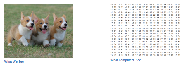
When a computer sees an image (accepts input data), it sees an array of pixels. Depending on the resolution and image size, for example, the size of the array can be 32x32x3 (where 3 is the values ​​of the RGB channels). To make it clearer, let's imagine, we have a color image in JPG format, and its size is 480x480. The corresponding array will be 480x480x3. Each of these numbers is assigned a value from 0 to 255, which describes the intensity of a pixel at this point. These figures, while remaining meaningless to us when we determine what is in the image, are the only input data available to the computer. The idea is that you give the computer this matrix, and it displays the numbers that describe the probability of the image class (.80 for cats, .15 for dogs, .05 for birds, etc.).

What do we want from the computer

Now that we have defined the task, the input and the output, let's think about how to approach the solution. We want the computer to be able to distinguish all the images given to it and recognize the unique features that make a dog a dog, and a cat a cat. We also have this process subconsciously. When we look at the image of a dog, we can relate it to a particular class, if the image has characteristic features that can be identified, such as legs or four legs. Similarly, a computer can classify images by searching for basic-level characteristics, such as borders and curvatures, and then building more abstract concepts through groups of convolutional layers. This is a general description of what the SNS is doing. We now turn to the specifics.

Biological connections

At the beginning of a little story. When you first heard the term convolutional neural networks, you might have thought about something related to neuroscience or biology, and were partly right. In a sense. SNS is really a prototype of the visual cortex. The visual cortex has small areas of cells that are sensitive to specific areas of the visual field. This idea was considered in detail with the help of the stunning experiment of Hubel and Wiesel in 1962 ( video ), in which they showed that individual brain nerve cells reacted (or activated) only with a visual perception of the boundaries of a particular orientation. For example, some neurons were activated when they perceived vertical boundaries, and some - horizontal or diagonal. Hubel and Wiesel found out that all these neurons are concentrated in the form of core architecture and together form a visual perception. This idea of ​​specialized components within the system that solve specific problems (as cells of the visual cortex that are looking for specific characteristics) and use machines, and this idea is the basis of the SNA.

Structure

Let's return to the specifics. What exactly are the SNS doing? An image is taken, passed through a series of convolutional, non-linear layers, merging layers and fully connected layers, and an output is generated. As we have said, the conclusion can be the class or probability of the classes that best describe the image. A difficult moment is an understanding of what each of these layers does. So let's move on to the most important.

The first layer is the mathematical part.

The first layer in the SNS is always convolutional. You remember what input is this convolutional layer? As mentioned earlier, the introductory image is a 32 x 32 x 3 matrix with pixel values. The easiest way to understand what a convolutional layer is if you imagine it in the form of a flashlight that shines on the upper left of the image. Suppose the light that this flashlight emits covers an area of ​​5 x 5. And now let's imagine that the flashlight moves in all areas of the introductory image. In terms of computer learning, this flashlight is called a filter (sometimes a neuron or a nucleus), and the areas to which it shines are called a receptive field (field of perception). That is, our filter is a matrix (such a matrix is ​​also called a weight matrix or parameter matrix). Note that the depth of the filter should be the same as the depth of the introductory image (then there is a guarantee of mathematical fidelity), and the dimensions of this filter are 5 x 5 x 3. Now let's take the position where the filter is located as an example. Let it be the upper left corner. Since the filter convolves, that is, moves through the introductory image, it multiplies the filter values ​​by the original pixel values ​​of the image (elementwise multiplication). All these multiplications are summed (total 75 multiplications). And as a result one number turns out. Remember, it simply symbolizes the location of the filter in the upper left corner of the image. Now we repeat this process in each position. (The next step is to move the filter right by one, then another one to the right, and so on). Each unique position of the entered image produces a number. After passing the filter through all positions, a matrix of 28 x 28 x 1 is obtained, which is called the activation function or feature map. The 28 x 28 matrix is ​​obtained because there are 784 different positions that can pass through a 5 x 5 filter, 32 x 32 images. These 784 numbers are converted into a 28 x 28 matrix.

(Small note: some of the images, including what you see above, are taken from Michael Nielsen’s stunning book “ Neural Networks and Deep Learning ” (“ Neural Networks and Deep Learning ” by Michael Nielsen). I highly recommend it).

Suppose now we use two 5 x 5 x 3 filters instead of one. Then the output value will be 28 x 28 x 2.

First layer

Let's talk about what this convolution actually does at a high level. Each filter can be viewed as a property identifier. When I say property, I mean straight borders, simple colors and curves. Think of the simplest features that have all the images in common. Let's say our first filter is 7 x 7 x 3, and it will be a curve detector. (Now let's ignore the fact that the filter has a depth of 3, and consider only the top layer of the filter and the image, for simplicity). The filter has a pixel structure, in which the numerical values ​​are higher along the area defining the shape of the curve (remember, the filters we are talking about are just numbers!).

Let's return to mathematical visualization. When we have a filter in the upper left corner of the introductory image, it multiplies the filter values ​​by the pixel values ​​of this area. Let's look at an example of an image to which we want to assign a class, and set the filter in the upper left corner.

Remember, all we need is to multiply the filter values ​​by the original pixel values ​​of the image.

In fact, if the introductory image has a form in general similar to the curve that this filter represents, and all the multiplied values ​​are added together, then the result will be a great value! Now let's see what happens when we move the filter.

The value is much lower! This is because there is nothing in the new image area that the curve definition filter could detect. Remember that the output of this convolutional layer is a property map. In the simplest case, if there is a single convolution filter (and if this filter is a curve detector), the property map will show areas in which there is more likelihood of curves. In this example, the value of our 28 x 28 x 1 property map in the upper left corner is 6600. This high value indicates that perhaps something like a curve is present in the image, and this possibility activated the filter. In the upper right corner, the value of the property map will be 0, because there was nothing in the picture that could activate the filter (in other words, there was no curve in this area). Remember that this is only for one filter. This is a filter that detects lines curved outward. There may be other filters for the lines bent inward or just straight. The more filters, the greater the depth of the property map, and the more information we have about the introductory picture.

Remark: The filter that I talked about in this section is simplified to simplify the folding mathematics. The figure below shows examples of actual visualizations of the filters of the first convolutional layer of the trained network. But the idea here is the same. The filters on the first layer are folded around the introductory image and "activated" (or produce large values) when the particular trait they are looking for is in the introductory image.

(Note: the images above are from the Stanford course 231N , which is taught by Andrei Karpaty and Justin Johnson. I recommend to those who want to learn more about SNS).

We go deeper in the network

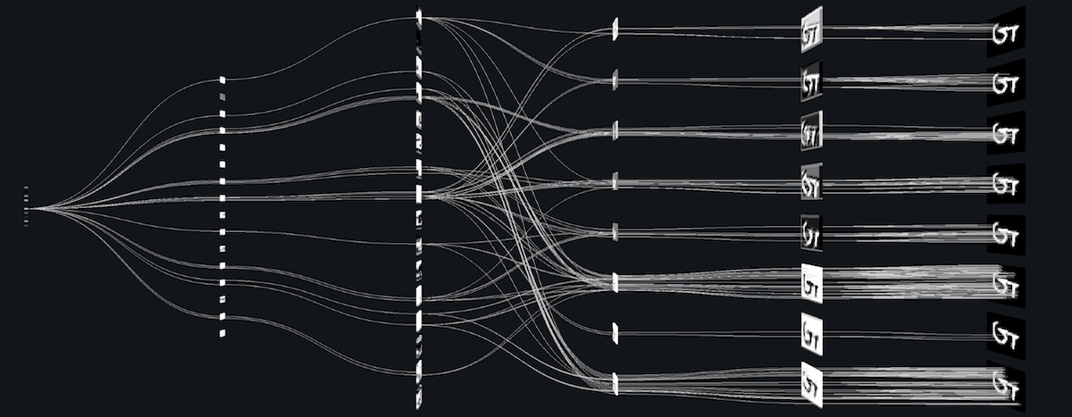
Today, in the traditional convolutional neural network architecture, there are other layers that are interspersed with convolutional layers. I highly recommend those interested in the topic to read about these layers in order to understand their functionality and effects. The classic architecture of the SNA will look like this:

The last layer, although at the end, is one of the most important - we will move on to it later. Let's summarize what we have already figured out. We talked about the fact that they are able to determine the filters of the first convolutional layer. They detect the properties of the base level, such as borders and curves. As you can imagine, in order to assume what type of object is depicted in the picture, we need a network that can recognize properties of a higher level, such as hands, paws, or ears. So let's think about what the output of the network looks like after the first convolutional layer. Its size is 28 x 28 x 3 (provided that we use three filters 5 x 5 x 3). When a picture passes through one convolutional layer, the output of the first layer becomes the introductory value of the 2nd layer. Now it's a little harder to visualize. When we talked about the first layer, the input was only the original image data. But when we went to the 2nd layer, the introductory value for it was one or more property maps - the result of processing the previous layer. Each set of input data describes the positions where certain basic features are found on the source image.

Now, when you apply a set of filters on top of this (skip the image through the second convolutional layer), the output will be activated filters that represent the properties of a higher level. The types of these properties can be half rings (a combination of a straight border with a bend) or squares (a combination of several straight edges). The more convolutional layers the image passes and the farther it travels through the network, the more complex characteristics are displayed in the activation maps. At the end of the network there may be filters that are activated when there is handwriting in the image, if there are pink objects, etc. If you want to learn more about convolutional network filters, Matt Seiler and Rob Fergus have written an excellent research paper on this topic. Also on YouTube there is a video of Jason Yoshinsky with an excellent visual presentation of these processes.

Another interesting point. When you move deeper into the network, the filters work with a larger field of perception, which means that they are able to process information from a larger area of ​​the original image (in simple words, they are better adapted to the processing of a larger area of ​​pixel space).

Fully connected layers

Now that we can detect high-level properties, the coolest thing is attaching a fully connected layer at the end of the network. This layer takes input data and outputs an N-spatial vector, where N is the number of classes from which the program selects the one you need. For example, if you want a program to recognize numbers, N will have a value of 10, because numbers are 10. Each number in this N-space vector represents the probability of a particular class. For example, if the resulting vector for the number recognition program is [0 0.1 0.1 0.75 0 0 0 0 0.05], then there is a 10% chance that the image is "1", 10% is the probability that the image "2", 75% probability - "3", and 5% probability - "9" (of course, there are other ways to present a conclusion).

The way that a fully connected layer works is to refer to the output of the previous layer (which, as we remember, should output high-level property maps) and the definition of properties that are more associated with a particular class. For example, if a program predicts that on some image of a dog, property maps that reflect high-level characteristics, such as legs or 4 legs, should have high values. In the same way, if the program recognizes that the image is a bird, it will have high values ​​in the property maps represented by high-level characteristics like wings or beak. The fully connected layer looks at the fact that high-level functions are strongly associated with a particular class and have certain weights, so when you calculate the products of weights with the previous layer, you get the correct probabilities for different classes.

Training (or "What makes this thing work")

This is one aspect of neural networks that I haven’t specifically mentioned so far. This is probably the most important part. Perhaps you have a lot of questions. Where do the filters of the first convolutional layer know what to look for borders and curves? How does a fully connected layer know what a property map is looking for? How do the filters of each layer know which values ​​to store? The way in which a computer is able to correct filter values ​​(or weights) is a learning process, which is called the backpropagation method.

Before proceeding to the explanation of this method, let's talk about what the neural network needs to work. When we are born, our heads are empty. We do not understand how to recognize a cat, dog or bird. The situation with the SNA is similar: until the network is built, the weights or values ​​of the filter are random. Filters do not know how to search for borders and curves. Filters of the upper layers do not know how to look for paws and beaks. When we get older, parents and teachers show us different pictures and images and assign them the appropriate labels. The same idea of ​​displaying a picture and assigning a label is used in the learning process that passes the SNA. Let's imagine that we have a set of training pictures in which thousands of images of dogs, cats and birds. Each image has a label with the name of the animal.

The backpropagation method can be divided into 4 separate blocks: forward distribution, loss function, back distribution and weight update. During direct propagation, a training image is taken — as you remember, this is a 32 x 32 x 3 matrix — and is passed through the entire network. In the first training example, since all weights or filter values ​​were initialized randomly, the output value will be something like [.1 .1 .1 .1 .1 .1 .1 .1 .1 .1], that is, a value that will not give preference to any particular number. The network with such weights cannot find the properties of the base level and cannot reasonably determine the class of the image. This leads to a loss function. Remember, what we use now is training data. Such data has both an image and a label. Suppose the first training image is the number 3. The image label will be [0 0 0 1 0 0 0 0 0 0]. The loss function can be expressed in different ways, but the mean-square deviation is often used (rms error), which is 1/2 multiplied by (reality - prediction) squared.

We take this value as the variable L. As you might guess, the loss will be very high for the first two training images. Now let's think about it intuitively. We want to ensure that the predicted label (the output of the convolutional layer) is the same as the label of the training image (this means that the network made the right assumption). To achieve this, we need to minimize the number of losses that we have. Visualizing this as an optimization problem from mathematical analysis, we need to figure out which inputs (weights, in our case) most directly contributed to the loss (or errors) of the network.

(One way to visualize the idea of ​​minimizing loss is a three-dimensional graph, where the neural network weights (obviously more than 2, but the example is simplified) are independent variables, and the dependent variable is loss. The task of minimizing losses is to adjust the weights so that to reduce the loss. Visually, we need to get closer to the lowest point of the cup-like object. To achieve this, we need to find the derivative of the loss (within the framework of the drawn graph, calculate the angular coefficient in each direction) taking into account the weights).

This is the mathematical equivalent of dL / dW , where W is the weight of a particular layer. Now we need to do backpropagation through the network, which determines which weights have had a greater impact on the losses, and find ways to adjust them to reduce the losses. After we calculate the derivative, we move on to the last stage - updating the weights. Take all filter weights and update them so that they change in the direction of the gradient.

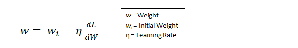
Learning speed is a parameter that is selected by the programmer. A high learning rate means that larger steps have been taken in weight updates, so the sample may take less time to gain an optimal set of weights. But too high a learning rate can lead to very large and insufficiently accurate jumps, which will prevent the achievement of optimal performance.

The forward propagation process, the loss function, the reverse propagation and updating of the weights, are commonly referred to as a single sampling period (or epoch - era). The program will repeat this process a fixed number of periods for each training image. After the update of parameters is completed on the last training sample, the network should in theory be well trained and the weights of the layers are set correctly.

Testing

Finally, to see if SNS works, we take a different set of images and shortcuts and skip the images through the network. We compare the outputs with the reality and see if our network works.

How companies use SNA

Data, data, data. Companies that have tons of this six-letter magical good, have a natural advantage over other competitors. The more training data that you can feed the network, the more you can create training iterations, more weight updates and before you go into production, get a better trained network. Facebook (and Instagram) can use all the photos of a billion users that they have today, Pinterest - information from 50 billion pins, Google - search data, and Amazon - data on millions of products that are bought daily. And now you know what kind of magic they use for their own purposes.

Remark

Although this post should be a good start for understanding the SNA, this is not a complete overview. Points that were not discussed in this article include nonlinear layers and pooling layers, as well as network hyper parameters, such as filter sizes, steps, and padding. Network architecture, packet normalization, fading gradients, fallout, initialization methods, non-convex optimization, shift, loss function variants, data expansion, regularization methods, machine features, backpropagation modifications, and many other unsupported (for now ;-) topics.

(Translation by Natalia Bass )