Graphic models based on Gaussian copulas
Log-linear models and their representations in the form of Markov networks allow us to show the structure of interrelations between random variables. However, the resulting visualization can be difficult to understand because of the large number of equivalent edges in the graph of such a model. When working with ordinal and binary variables, Gaussian copulas (Gaussian copula graphical models, abbr. GCGM) make it possible to increase the visibility and simplify the interpretation of the model. The article provides a brief overview of the theory and built an example of GCGM for European Social Survey data.
In one of the previous articles , which dealt with log-linear models and Markov networks, a comic example of the relationship between the size of a man’s shoes and his mathematical abilities was considered. Statistical tests suggest that, as a rule, people with a larger shoe size have higher mathematical abilities.
Consider a real example - the study of the "European customer satisfaction index with the mobile services market" for 2005. The data is available in the semPLS package of the R environment. Each survey variable represents a rating with a scale from 1 to 10. Of these data, we consider only three variables — the mobile provider’s rating when recommending it to friends or colleagues (Recommendation); evaluation of the reasonableness of service fees (Fair Price); assessment of the quality of services provided by the mobile operator (Overall Quality). A summary of the survey results for these variables is shown below.
')

To assess the degree of association between the variables of Recommendation and Fair Price, we use the Spearman correlation coefficient. It turns out quite large.

If we consider all three variables together and find their partial correlations - pairwise correlation coefficients, taking into account the influence of the third variable, the result is different.

Note that the correlation coefficient between the Recommendation and Fair Price variables, taking into account the influence of the Overall Quality variable, turned out to be very small. The pair correlation between these variables, equal to 0.4, decreased, in the case of partial correlation between them, to 0.02.
The matrix obtained above determines the next graph with edge weights equal to partial correlation coefficients.

Everything seemed to be good, however, the zero (or close to zero) coefficient of partial correlation between random variables, in general, does not indicate that these random variables are conditionally independent. However, this property is valid for multidimensional normally distributed random variables. That is, two one-dimensional random variables from the distribution conditionally independent if and only if their partial correlation coefficient is zero. Equality zero ( i, j ) of the coefficient of partial correlation is equivalent to the equality to zero ( i, j ) of the matrix element inverse to
  . Matrix Evaluation
  or rather its sparse form, is the main object of modeling in the construction of Gaussian graphical models (gaussian graphical models / gaussian markov random fields).
The above survey data on the estimates of the services of mobile service providers cannot be considered as a sample of a 3-dimensional normally distributed random variable. Is it possible for such data to build a graphical model taking into account the partial correlation coefficients? The answer is yes. For these purposes, the simulation of Gaussian copulas is suitable.
Before we talk about Gaussian copulas, a few words about the general construction. Suppose there is a set of cumulative observations of several variables (random variables). The distribution functions of each of these random variables separately - one-dimensional marginal distributions, do not say anything about the relationships between variables. This information is determined by the joint distribution of random variables.
Copula is a function that relates the joint distribution of random variables and their marginal distributions (hereafter, only one-dimensional marginal distributions are meant everywhere). The exact definition in Russian can be found in [1]. What is the attractiveness of copulas? I will quote [1]: “Copula functions make it possible to divide the description of the distribution of a random vector into two parts: particular component distributions and the structure of their dependencies.”
If some of the marginal distributions of a copula are discrete, then there are certain difficulties in assessing such a copula. The reason for this situation is the absence of a one-to-one correspondence between the region of values of k marginal random variables and the domain of definition of the copula — the hypercube . Details can be found, for example, in review [2].
Gaussian copula has the form:

Where - k -dimensional normal distribution function with zero mean vector and correlation matrix ,
  - quantile function of the standard normal distribution. This formula performs a double conversion of variables. Let be
  the observed value of the random variable in the first coordinate, and
  - marginal distribution function (cdf) of this random variable. Then we assume
  and we get the value
  the latent variable of the first coordinate of the k- dimensional Gaussian distribution.
In article [3] several examples of Gaussian copulas with both continuous and discrete marginal random variables are considered in detail. In general, Gaussian copulas should not be taken solely in the context of a tool for Markov networks. As can be seen from the work of Danaher and Smith, these are also methods for building models of consumer activity and finding the distribution of coverage (Reach distribution) of an advertising campaign in the media and a number of other models of joint distribution of random variables. An analysis of one of these examples with the code for R can be found below under the spoiler.
The problem of estimating the parameters of GCGM can be divided into two parts - finding the correlation matrix of a Gaussian copula and obtaining a sparse matrix from it for a graphical representation. As before, we will consider the method as applied to survey data. One of the features of such data is the use of weights. Therefore, in the general case, it is required to take into account the sample weights when estimating the model parameters.
There are several methods for estimating Gaussian copulas with discrete (or with discrete and continuous) marginal distributions. One of them was proposed by Hoff in [4] and implemented by him in the R sbgcop library. This algorithm can be adapted to the weighted data, taking into account the sample weights when determining the rank marginal empirical distribution functions.
Here, too, there is room for choice. When the correlation matrix of a Gaussian copula is obtained, you can use the classic glasso library algorithm based on the article [5]. Another approach was proposed in [6] and implemented by the authors in the R BDgraph library. This method assumes a joint assessment of both matrices - the correlation matrix of a Gaussian copula and the sparse matrix of a graphical model at each step of the algorithm iteration.
The first library is written entirely in R and contains several nested for-cycles. That is, the calculations are organized inefficiently. In addition, sampling from a truncated normal distribution is implemented numerically unstable by the Inverse Transform method. Under certain conditions, quite probable in practical application, instead of the sampled value, Inf.
Most of the second library is written in C ++, where all for-cycles from sbgcop have been transferred, in particular. Linear algebra is written using Fortran. The problem with sampling from a truncated normal distribution is also relevant in this package.
Graphic models based on Gaussian copulas can be used with a variety of data - marketing, sociological, biological, and many others. Here we look at the data of the European Social Survey for 2012 - ESS Round 6 European Social Survey Round 6 Data (data file edition 2.2), which are freely available ( link ). From this data we select only respondents from Russia. In the “Policy” block of this survey, the following 5 assessment judgments about the degree of trust to various political bodies and institutions of power are presented.

where the scale varies from 0 = No trust at all to 10 = Complete trust.
Let's add this set of values with the following four variables:
We select respondents aged 23 years and over who have no missing values in the answers to all the questions under consideration. The model also uses the weight of the respondents of the study - design weight.
An out-of-the-box solution is available for building a model graph — the qgraph function of the library of the same name builds an image of a graphical model defined by a partial correlation matrix. A more flexible and visual solution can be achieved using the R packages visNetwork (uses the JS library vis.js) and shiny. The first package performs the construction of the model graph, the second complements the ability to adjust the level of sparseness of the model on the fly.

The picture is clickable, the link leads to the html file with the graph of the model.
Here, the Normalized Sparsity Level is responsible for the value of the coefficient before the L1 norm of the penalty function of the graphical lasso problem (these values are normalized so that the minimum value of the coefficient at which the graph of the model does not contain edges is set to 1). The second control parameter, Absolute Correlation Level, hides edges between vertices, in which the partial correlation coefficients are in absolute value less than the specified value.
In the snapshot with the graph, the value of the edge weight between the vertices of voted is highlighted (1 - voted, 2 - no) and interested in politics (1 - not at all, ..., 4 - definitely yes). This value of -0.34 shows a rather strong level of association between interest in politics and readiness to vote in elections, which is quite expected.
Another picture:
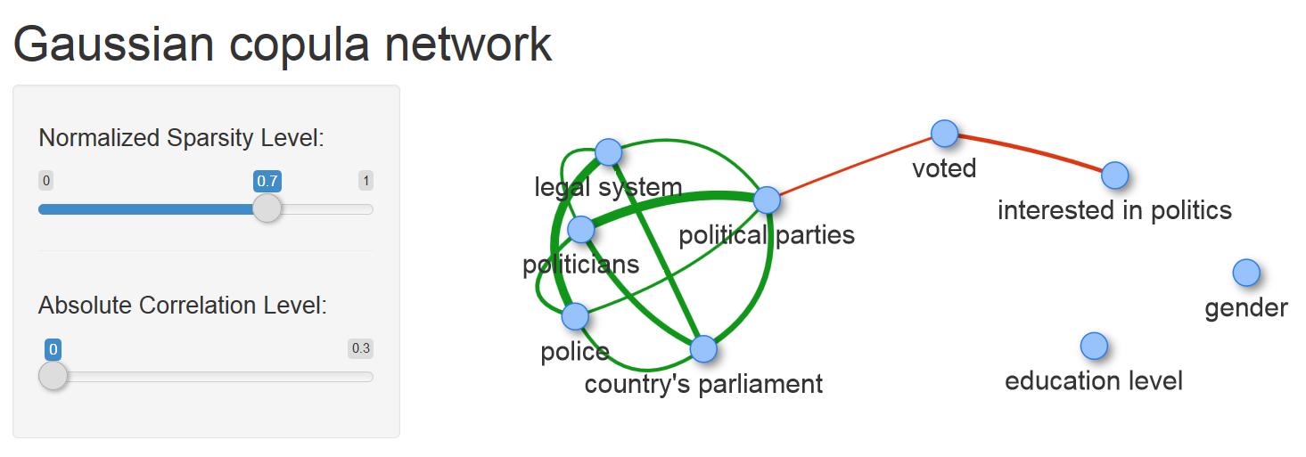
I think the most important part of this model is the edge connecting the tops of voted and political parties. It only connects the two components of the graph and the decision to participate in the voting at elections directly depends on only one trust variable - trust in political parties. All other trust variables are conditionally independent with the variable voted. Therefore, among the variables considered, this bundle is a key factor in the interaction of citizens and the state.
Not in all cases there is an a priori choice of a set of variables for building a model. If it is of interest to build a GCGM in which graph any particular variable will be included, what additional variables should be selected for analysis?
Too many input variables for GCGM have two problems. First, finding the parameters of a Gaussian copula for discrete data is a time-consuming computational process. The power of the laptop to solve a problem with a large number of variables in an acceptable time will not be enough. Secondly, the understanding of a graph with a large number of variables, albeit sparse, will be difficult (for example, the strong connections of any variables that are completely uninteresting in the context of the task in question) can “interfere”.
A suitable solution to the issue of selecting variables in GCGM for a given variable is to build a minimum mutual information tree (Chow-Liu tree). This is a fast algorithm, the description of which is not included in my plans in this publication. Details can be found in article [7]. The structural property of the Chow-Liu tree, loosely speaking, is as follows: the closer the two vertices in this tree are to one another, the more “dependent” they are. Therefore, we find the target variable in the tree, determine the radius, and select all suitable vertices of this tree. The example below is built for the target variable “In Russia, political parties offer voters truly different programs”, with a response scale from 0 to 10. The example tree was built using the NetworkD3 R library (creates a series of d3.js graphs).
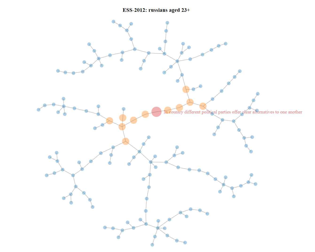
The picture is clickable, the link leads to the html file.
The GCGM method, supplemented by a pre-selection algorithm for variables, allows you to quickly, easily and meaningfully analyze the structure of dependencies in the data, highlighting key relationships in them.
[1] D. Fantazzini (2011) Modeling of multidimensional distributions using copula functions. I, Applied Econometrics, 2 (22), 98 - 134.
[2] C. Genest and J. Nešlehová (2007) A Primer on Copulas for Count Data, ASTIN Bulletin, 37 (2), pp. 475-515.
[3] PJ Danaher and MS Smith (2011) Modeling Multivariate Distributions of Copulas: Applications in Marketing, Marketing Science 30 (1), pp. 4-21.
[4] PD Hoff (2007) Extending the rank likelihood for semiparametric copulamination, Ann. Appl. Stat., 1, pp. 265-283.
[5] J. Friedman, T. Hastie and R. Tibshirani (2008) Sparse inverse covariance assessment with the lasso, Biostatistics, 9 (3), pp. 432–441
[6] A. Mohammadi and EC Wit (2015) Bayesian Structure Learning in Sparse Gaussian Graphic Models, Bayesian Anal. 10 (1), pp. 109-138.
[7] D. Edwards, GCG de Abreu and R. Labouriau (2010). Selecting high-dimensional mixed graphical models using minimal AIC or BIC forests. BMC Bioinformatics, 11:18.
UPD: a small piece of text was omitted with the words that the Gaussian graphical model is not suitable for the presentation of the data under consideration - the last paragraph of the section "Partial correlation and conditional independence".
Partial correlation and conditional independence
In one of the previous articles , which dealt with log-linear models and Markov networks, a comic example of the relationship between the size of a man’s shoes and his mathematical abilities was considered. Statistical tests suggest that, as a rule, people with a larger shoe size have higher mathematical abilities.
Consider a real example - the study of the "European customer satisfaction index with the mobile services market" for 2005. The data is available in the semPLS package of the R environment. Each survey variable represents a rating with a scale from 1 to 10. Of these data, we consider only three variables — the mobile provider’s rating when recommending it to friends or colleagues (Recommendation); evaluation of the reasonableness of service fees (Fair Price); assessment of the quality of services provided by the mobile operator (Overall Quality). A summary of the survey results for these variables is shown below.
')
To assess the degree of association between the variables of Recommendation and Fair Price, we use the Spearman correlation coefficient. It turns out quite large.
If we consider all three variables together and find their partial correlations - pairwise correlation coefficients, taking into account the influence of the third variable, the result is different.
Note that the correlation coefficient between the Recommendation and Fair Price variables, taking into account the influence of the Overall Quality variable, turned out to be very small. The pair correlation between these variables, equal to 0.4, decreased, in the case of partial correlation between them, to 0.02.
The matrix obtained above determines the next graph with edge weights equal to partial correlation coefficients.
But ....
Everything seemed to be good, however, the zero (or close to zero) coefficient of partial correlation between random variables, in general, does not indicate that these random variables are conditionally independent. However, this property is valid for multidimensional normally distributed random variables. That is, two one-dimensional random variables from the distribution
conditionally independent if and only if their partial correlation coefficient is zero. Equality zero ( i, j ) of the coefficient of partial correlation is equivalent to the equality to zero ( i, j ) of the matrix element inverse to . Matrix Evaluation or rather its sparse form, is the main object of modeling in the construction of Gaussian graphical models (gaussian graphical models / gaussian markov random fields).The above survey data on the estimates of the services of mobile service providers cannot be considered as a sample of a 3-dimensional normally distributed random variable. Is it possible for such data to build a graphical model taking into account the partial correlation coefficients? The answer is yes. For these purposes, the simulation of Gaussian copulas is suitable.
Something about copulas
Before we talk about Gaussian copulas, a few words about the general construction. Suppose there is a set of cumulative observations of several variables (random variables). The distribution functions of each of these random variables separately - one-dimensional marginal distributions, do not say anything about the relationships between variables. This information is determined by the joint distribution of random variables.
Copula is a function that relates the joint distribution of random variables and their marginal distributions (hereafter, only one-dimensional marginal distributions are meant everywhere). The exact definition in Russian can be found in [1]. What is the attractiveness of copulas? I will quote [1]: “Copula functions make it possible to divide the description of the distribution of a random vector into two parts: particular component distributions and the structure of their dependencies.”
If some of the marginal distributions of a copula are discrete, then there are certain difficulties in assessing such a copula. The reason for this situation is the absence of a one-to-one correspondence between the region of values of k marginal random variables and the domain of definition of the copula — the hypercube
. Details can be found, for example, in review [2].Gaussian copula
Gaussian copula has the form:
Where
- k -dimensional normal distribution function with zero mean vector and correlation matrix , - quantile function of the standard normal distribution. This formula performs a double conversion of variables. Let be the observed value of the random variable in the first coordinate, and - marginal distribution function (cdf) of this random variable. Then we assume and we get the value the latent variable of the first coordinate of the k- dimensional Gaussian distribution.In article [3] several examples of Gaussian copulas with both continuous and discrete marginal random variables are considered in detail. In general, Gaussian copulas should not be taken solely in the context of a tool for Markov networks. As can be seen from the work of Danaher and Smith, these are also methods for building models of consumer activity and finding the distribution of coverage (Reach distribution) of an advertising campaign in the media and a number of other models of joint distribution of random variables. An analysis of one of these examples with the code for R can be found below under the spoiler.
Hidden text
Consider a simple example from article [3] - a survey on the frequency of purchases of eggs and bacon for the last four visits to the supermarket. The method for estimating the parameter of a Gaussian copula modeling the input data, which is given in the code below, differs from the one proposed in the article. It uses the Hoff rank method, which will be discussed in the next paragraph. The task is to build a function, a Gaussian copula, simulating this joint distribution based on the input data on the joint distribution of the number of purchases of eggs and bacon.
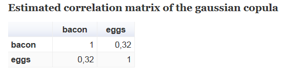
We obtain a sufficiently large positive correlation coefficient between the number of purchases of eggs and bacon. Now compare the original figures with the results obtained by modeling the Gaussian copula

In the picture above, the table on the left is the input data with the results of the customer survey; the table on the right shows the results obtained by modeling the input data with a Gaussian copula. For example, among all 548 survey respondents, 16 (2.9%) bought bacon 1 time and eggs 2 times. The model estimates the number of such buyers at 15.18 (2.8%).
Mosaic table graphics

require(MM) # to load the example data data(danaher) # define data sample corresponding to the contingency table df.danaher<-data.frame( bacon=rep(0:4,rowSums(danaher)), eggs=unlist(apply( danaher, 1, function(x) rep(0:4, x) )) ) # fit the gaussian copula require(sbgcop) fit <- sbgcop.mcmc(df.danaher, nsamp = 5000, odens = 1, seed = 1, verb = F) # estimate the correlation matrix burn.in <- 500 Sigma <- apply(fit$C.psamp[,,-c(1:burn.in)], c(1,2), median) # find the fitted results n <- nrow(danaher) N <- sum(danaher) eggs.cum.sum <- cumsum( colSums(danaher)/N ) bacon.cum.sum <- cumsum( rowSums(danaher)/N ) eggs.norm.limits <- qnorm( c(0, eggs.cum.sum) ) bacon.norm.limits <- qnorm( c(0, bacon.cum.sum) ) lower.limits <- as.matrix( expand.grid(head(eggs.norm.limits, n), head(bacon.norm.limits, n)) ) upper.limits <- as.matrix( expand.grid(tail(eggs.norm.limits, n), tail(bacon.norm.limits, n)) ) require(mvtnorm) # to the distribution function of the multivariate normal distribution fitted.results <- sapply(1:n^2, function(i) pmvnorm(lower.limits[i,], upper.limits[i,], corr = Sigma)*N) fitted.results <- matrix(fitted.results, nrow = 5, byrow = T) dimnames(fitted.results) <- list(bacon = as.character(0:4), eggs = as.character(0:4)) # Estimated correlation matrix of the gaussian copula Sigma # Input data danaher # Fitted results fitted.results # Mosaic plots of the input data and fitted results par(mfrow = c(1,2)) mosaicplot(t(danaher), main = "Input data", color = "royalblue") mosaicplot(t(fitted.results), main = "Fitted results", color = "royalblue") Results:
We obtain a sufficiently large positive correlation coefficient between the number of purchases of eggs and bacon. Now compare the original figures with the results obtained by modeling the Gaussian copula
In the picture above, the table on the left is the input data with the results of the customer survey; the table on the right shows the results obtained by modeling the input data with a Gaussian copula. For example, among all 548 survey respondents, 16 (2.9%) bought bacon 1 time and eggs 2 times. The model estimates the number of such buyers at 15.18 (2.8%).
Mosaic table graphics
Estimation of parameters of a graphical model of a Gaussian copula
The problem of estimating the parameters of GCGM can be divided into two parts - finding the correlation matrix of a Gaussian copula and obtaining a sparse matrix from it for a graphical representation. As before, we will consider the method as applied to survey data. One of the features of such data is the use of weights. Therefore, in the general case, it is required to take into account the sample weights when estimating the model parameters.
Estimation of the correlation matrix of a Gaussian copula
There are several methods for estimating Gaussian copulas with discrete (or with discrete and continuous) marginal distributions. One of them was proposed by Hoff in [4] and implemented by him in the R sbgcop library. This algorithm can be adapted to the weighted data, taking into account the sample weights when determining the rank marginal empirical distribution functions.
Obtaining a sparse matrix of a graphical model of a gaussian copula
Here, too, there is room for choice. When the correlation matrix of a Gaussian copula is obtained, you can use the classic glasso library algorithm based on the article [5]. Another approach was proposed in [6] and implemented by the authors in the R BDgraph library. This method assumes a joint assessment of both matrices - the correlation matrix of a Gaussian copula and the sparse matrix of a graphical model at each step of the algorithm iteration.
Comments on sbgcop (v.0.975) and BDgraph libraries (v.2.27)
The first library is written entirely in R and contains several nested for-cycles. That is, the calculations are organized inefficiently. In addition, sampling from a truncated normal distribution is implemented numerically unstable by the Inverse Transform method. Under certain conditions, quite probable in practical application, instead of the sampled value, Inf.
Most of the second library is written in C ++, where all for-cycles from sbgcop have been transferred, in particular. Linear algebra is written using Fortran. The problem with sampling from a truncated normal distribution is also relevant in this package.
GCGM usage example
Graphic models based on Gaussian copulas can be used with a variety of data - marketing, sociological, biological, and many others. Here we look at the data of the European Social Survey for 2012 - ESS Round 6 European Social Survey Round 6 Data (data file edition 2.2), which are freely available ( link ). From this data we select only respondents from Russia. In the “Policy” block of this survey, the following 5 assessment judgments about the degree of trust to various political bodies and institutions of power are presented.
where the scale varies from 0 = No trust at all to 10 = Complete trust.
Let's add this set of values with the following four variables:
- "How interested in politics" with 4 categories (1 - Not at all interested, ..., 4 - Very interested);
- “Did you vote in the last national election?” With 2 categories (1 - Yes, 2 - No), the question referred to voting in elections to the State Duma of the Russian Federation in 2011;
- "Gender" (1 - Male, 2 - Female)
- “Education” with 11 categories (1- No primary, ..., 11 - Ph.D.).
We select respondents aged 23 years and over who have no missing values in the answers to all the questions under consideration. The model also uses the weight of the respondents of the study - design weight.
An out-of-the-box solution is available for building a model graph — the qgraph function of the library of the same name builds an image of a graphical model defined by a partial correlation matrix. A more flexible and visual solution can be achieved using the R packages visNetwork (uses the JS library vis.js) and shiny. The first package performs the construction of the model graph, the second complements the ability to adjust the level of sparseness of the model on the fly.
The picture is clickable, the link leads to the html file with the graph of the model.
Here, the Normalized Sparsity Level is responsible for the value of the coefficient before the L1 norm of the penalty function of the graphical lasso problem (these values are normalized so that the minimum value of the coefficient at which the graph of the model does not contain edges is set to 1). The second control parameter, Absolute Correlation Level, hides edges between vertices, in which the partial correlation coefficients are in absolute value less than the specified value.
In the snapshot with the graph, the value of the edge weight between the vertices of voted is highlighted (1 - voted, 2 - no) and interested in politics (1 - not at all, ..., 4 - definitely yes). This value of -0.34 shows a rather strong level of association between interest in politics and readiness to vote in elections, which is quite expected.
Another picture:
What does the model show?
I think the most important part of this model is the edge connecting the tops of voted and political parties. It only connects the two components of the graph and the decision to participate in the voting at elections directly depends on only one trust variable - trust in political parties. All other trust variables are conditionally independent with the variable voted. Therefore, among the variables considered, this bundle is a key factor in the interaction of citizens and the state.
Selection of variables to build GCGM
Not in all cases there is an a priori choice of a set of variables for building a model. If it is of interest to build a GCGM in which graph any particular variable will be included, what additional variables should be selected for analysis?
Too many input variables for GCGM have two problems. First, finding the parameters of a Gaussian copula for discrete data is a time-consuming computational process. The power of the laptop to solve a problem with a large number of variables in an acceptable time will not be enough. Secondly, the understanding of a graph with a large number of variables, albeit sparse, will be difficult (for example, the strong connections of any variables that are completely uninteresting in the context of the task in question) can “interfere”.
A suitable solution to the issue of selecting variables in GCGM for a given variable is to build a minimum mutual information tree (Chow-Liu tree). This is a fast algorithm, the description of which is not included in my plans in this publication. Details can be found in article [7]. The structural property of the Chow-Liu tree, loosely speaking, is as follows: the closer the two vertices in this tree are to one another, the more “dependent” they are. Therefore, we find the target variable in the tree, determine the radius, and select all suitable vertices of this tree. The example below is built for the target variable “In Russia, political parties offer voters truly different programs”, with a response scale from 0 to 10. The example tree was built using the NetworkD3 R library (creates a series of d3.js graphs).
The picture is clickable, the link leads to the html file.
Summary
The GCGM method, supplemented by a pre-selection algorithm for variables, allows you to quickly, easily and meaningfully analyze the structure of dependencies in the data, highlighting key relationships in them.
Literature
[1] D. Fantazzini (2011) Modeling of multidimensional distributions using copula functions. I, Applied Econometrics, 2 (22), 98 - 134.
[2] C. Genest and J. Nešlehová (2007) A Primer on Copulas for Count Data, ASTIN Bulletin, 37 (2), pp. 475-515.
[3] PJ Danaher and MS Smith (2011) Modeling Multivariate Distributions of Copulas: Applications in Marketing, Marketing Science 30 (1), pp. 4-21.
[4] PD Hoff (2007) Extending the rank likelihood for semiparametric copulamination, Ann. Appl. Stat., 1, pp. 265-283.
[5] J. Friedman, T. Hastie and R. Tibshirani (2008) Sparse inverse covariance assessment with the lasso, Biostatistics, 9 (3), pp. 432–441
[6] A. Mohammadi and EC Wit (2015) Bayesian Structure Learning in Sparse Gaussian Graphic Models, Bayesian Anal. 10 (1), pp. 109-138.
[7] D. Edwards, GCG de Abreu and R. Labouriau (2010). Selecting high-dimensional mixed graphical models using minimal AIC or BIC forests. BMC Bioinformatics, 11:18.
UPD: a small piece of text was omitted with the words that the Gaussian graphical model is not suitable for the presentation of the data under consideration - the last paragraph of the section "Partial correlation and conditional independence".
Source: https://habr.com/ru/post/309182/
All Articles