Optimization by example. Imitation annealing against the ant algorithm. Part 1
Good day to all. Recently I read an article about imitation annealing on the example of the traveling salesman problem. The picture before and after optimization caused interest. Something like this is lured. Also in the comments I noticed that it would be interesting for people to look at the comparison with other types of optimization.
I like the Habr site, especially I like the way people know how to correctly express their "technical" thoughts on paper, which I cannot say about myself. Therefore, I tried to describe everything as much as possible in the comments - it is much easier for me, and it will be more convenient for you to understand.
The code is written in MATLAB. With a specific spelling syntax is easy to understand. When writing algorithms, I tried to maintain a balance between the “understanding” of the code and the speed of execution, eliminating vectorization, and where it is — alternative code was written in the comments. If you have any questions - I will try to answer in the comments. This is the first part of the series “Optimization by Example”; further publications will be published depending on your comments. That is, if you need a comparison with other heuristic methods, or if you have any suggestion (say, change the temperature formula, or the initial location of ants), where you can refine, and where you can change part of the algorithm, write. It will be interesting to everyone, and me too. I implement and publish as much as possible.
')
The purpose of the publication, first of all, to show on the detailed comments in the code the principle of operation of the two algorithms, the comparison is a secondary goal. In this article, comparing “purely” will not work, since the two algorithms, especially formic, contain a decent number of initial variable parameters. Moreover, some questions arose, but more on that later. In the simulation annealing easier, however, also has its own nuances. For those who are just familiar with these algorithms, I recommend first reading the useful material located at the end of the article.
The theory of two algorithms is on Habré and on other sites, but I didn’t find the open code of the ant algorithm with explanatory comments, there is pseudo-code, there are separate parts of it. The code of imitation annealing on MATLAB was laid out earlier, however, for comparison with other types of optimization, it has a low speed. Therefore, I wrote my own, increasing the speed at times. Both algorithms are written without built-in eigenfunctions, because with a small code, in my opinion, it is easier to perceive the structure of the algorithm. In places where you can get confused tried to give more detailed comments. Proceeding from this, I will not go into the theory, I will give only the following:
The method of simulating annealing reflects the behavior of the material body during controlled cooling. Studies have shown that during solidification of the molten material, its temperature should decrease gradually, until the moment of complete crystallization. If the cooling process proceeds too quickly, significant irregularities in the structure of the material are formed, which cause internal stresses. Rapid fixation of the energy state of the body at a level above the normal is similar to the convergence of the optimization algorithm to the local minimum point. The energy of the state of the body corresponds to the objective function, and the absolute minimum of this energy - the global minimum [1] .
One of the efficient polynomial algorithms for finding approximate solutions to the traveling salesman problem, as well as solving similar route search problems on graphs. The essence of the approach lies in the analysis and use of the model of the behavior of ants looking for paths from the colony to the power source and represents a meta-heuristic optimization [2] .
There are many modifications of ant algorithms. Somewhere a different update of pheromones, somewhere there are "elite" ants, and somewhere a different location of the ants at the start. In the code, just comment out something, uncomment something.
So, let's compare, we will generate for the beginning 30 cities.
Imitation annealing:
Options:
Now look at the work of the ant algorithm at the same coordinates.
Ant algorithm:
Options:
Before you visual work of two algorithms. Once again I will note that a detailed explanation (especially of the ant algorithm) in the comments of the code.
Please note that in imitation annealing, the optimum was already found at 20,000 iterations, then, when the temperature was low enough, the probability of switching to new routes decreased significantly, so the algorithm “got up”. Here you can enter the criteria for stopping. The higher the initial temperature, the greater the likelihood of getting to the optimal route, and the more iterations will be performed, however, it is far from a fact that we will find a global optimum.
In the ant algorithm, everything is different. The main advantage of the ant algorithm is that it will never stop, it will always look for better ways. With an infinite number of iterations (generations), the probability of finding a global optimum will tend to 1. However, at the very beginning the question arose: which initial parameters should we choose? Answer: the method of selection. We are optimizing again. These parameters of the ant optimization were optimized using a genetic algorithm not at these coordinates . There were other coordinates and the number of cities was 50. Not really getting good convergence, I got some parameters that roughly correspond to this example.
On one test, I did not go far, so I bring a table from a series of tests.

One can see the stability of the two algorithms, however, the variation in the mean value of the ant algorithm is smaller.
Now let's look at the work of two algorithms per 100 generated cities.
Imitation annealing:
Options:
Now look at the work of the ant algorithm at the same coordinates.
Ant algorithm:
Options:
Here the parameters took "by eye".
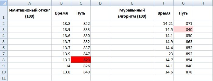
Again, the ant algorithm showed a better result, however, let's look again at the table from the test series:
Here imitative annealing went far ahead. In general, before I read the article, I was skeptical about imitative annealing. In the development of trading systems (in which I am involved) and their optimization, the annealing method is not suitable, since it is not the local optimum itself that is important for us, but the “spread” around it. On a conditional example: there is a moving average of 15 days on some paper, the yield for the year showed 10,000, and at 14 days (-1000). Here it is important for us that near the optimal parameter the profit should evenly decrease. Therefore, in different situations - different optimization.
As for the traveling salesman task, I, even if not in a “pure” competition (because it didn’t work out the right parameters for the ant algorithm), give up the victory to simulated annealing. If you add a stopping criterion, the same distances can be achieved in 2.5 seconds without much changing the standard deviation, which is not the case with the ant algorithm. According to a series of tests, much of which did not get here, the ant algorithm works brilliantly up to 50 cities, then begins to "drizzle", the optimization time slows down dramatically, which is logical in principle. However, he confidently goes to the global optimum, even if slowly.
Somewhere deep in my heart I still want the ant algorithm to show itself better. Maybe that is why the feeling that I made a mistake somewhere, and not just one, does not leave. Therefore, those who are interested, and those who are just starting their way in this direction - join. Write comments with suggestions, both about the algorithms, and about how best to submit the material.
In the meantime, look at today's winner. 500 cities, 86 seconds of optimization (and this is far from the limit).
Very cool!
Catch up or not the ant algorithm? Will it overtake it genetic? Who will be more effective? About this and another in the following publications.
Useful material:
» Video about ant algorithm (in Russian)
» Video about imitation annealing (in Russian)
» An article about the ant algorithm (in Russian)
» An article about imitation annealing (in Russian)
I like the Habr site, especially I like the way people know how to correctly express their "technical" thoughts on paper, which I cannot say about myself. Therefore, I tried to describe everything as much as possible in the comments - it is much easier for me, and it will be more convenient for you to understand.
The code is written in MATLAB. With a specific spelling syntax is easy to understand. When writing algorithms, I tried to maintain a balance between the “understanding” of the code and the speed of execution, eliminating vectorization, and where it is — alternative code was written in the comments. If you have any questions - I will try to answer in the comments. This is the first part of the series “Optimization by Example”; further publications will be published depending on your comments. That is, if you need a comparison with other heuristic methods, or if you have any suggestion (say, change the temperature formula, or the initial location of ants), where you can refine, and where you can change part of the algorithm, write. It will be interesting to everyone, and me too. I implement and publish as much as possible.
')
The purpose of the publication, first of all, to show on the detailed comments in the code the principle of operation of the two algorithms, the comparison is a secondary goal. In this article, comparing “purely” will not work, since the two algorithms, especially formic, contain a decent number of initial variable parameters. Moreover, some questions arose, but more on that later. In the simulation annealing easier, however, also has its own nuances. For those who are just familiar with these algorithms, I recommend first reading the useful material located at the end of the article.
The theory of two algorithms is on Habré and on other sites, but I didn’t find the open code of the ant algorithm with explanatory comments, there is pseudo-code, there are separate parts of it. The code of imitation annealing on MATLAB was laid out earlier, however, for comparison with other types of optimization, it has a low speed. Therefore, I wrote my own, increasing the speed at times. Both algorithms are written without built-in eigenfunctions, because with a small code, in my opinion, it is easier to perceive the structure of the algorithm. In places where you can get confused tried to give more detailed comments. Proceeding from this, I will not go into the theory, I will give only the following:
Imitation annealing
The method of simulating annealing reflects the behavior of the material body during controlled cooling. Studies have shown that during solidification of the molten material, its temperature should decrease gradually, until the moment of complete crystallization. If the cooling process proceeds too quickly, significant irregularities in the structure of the material are formed, which cause internal stresses. Rapid fixation of the energy state of the body at a level above the normal is similar to the convergence of the optimization algorithm to the local minimum point. The energy of the state of the body corresponds to the objective function, and the absolute minimum of this energy - the global minimum [1] .
Ant algorithm
One of the efficient polynomial algorithms for finding approximate solutions to the traveling salesman problem, as well as solving similar route search problems on graphs. The essence of the approach lies in the analysis and use of the model of the behavior of ants looking for paths from the colony to the power source and represents a meta-heuristic optimization [2] .
There are many modifications of ant algorithms. Somewhere a different update of pheromones, somewhere there are "elite" ants, and somewhere a different location of the ants at the start. In the code, just comment out something, uncomment something.
Imitation annealing. Full code with comments
% ( ) %-------------------------------------------------------------------------- tic % clearvars -except cities clearvars % ----------------------------------------------------------------- % - m = 100000; % ---------------------------------------------------------------- % Tstart = 10000; % Tend = 0.1; % T = Tstart; % S = inf; % n = 100; % ------------------------------------------------------------------- % dist = zeros(n,n); % ------------------------------------------------------------------------- % (x,y) cities = rand(n,2)*100; % ROUTE = randperm(n); % for i = 1:n for j = 1:n % dist ( ) dist(i,j) = sqrt((cities(i,1) - cities(j,1))^2 + ... (cities(i,2) - cities(j,2))^2); end end % , - for k = 1:m % Sp = 0; % , ROUTEp - % % ROUTEp = ROUTE; % transp = randperm(n,2); % , transp % if transp(1) < transp(2) ROUTEp(transp(1):transp(2)) = fliplr(ROUTEp(transp(1):transp(2))); else ROUTEp(transp(2):transp(1)) = fliplr(ROUTEp(transp(2):transp(1))); end % () for i = 1:n-1 Sp = Sp + dist(ROUTEp(i),ROUTEp(i+1)); end Sp = Sp + dist(ROUTEp(1),ROUTEp(end)); % , ... % , , if Sp < S S = Sp; ROUTE = ROUTEp; else % 0 1 RANDONE = rand(1); % P = exp((-(Sp - S)) / T); if RANDONE <= P S = Sp; ROUTE = ROUTEp; end end % T = Tstart / k; % if T < Tend break; end; end % citiesOP(:,[1,2]) = cities(ROUTE(:),[1,2]); plot([citiesOP(:,1);citiesOP(1,1)],[citiesOP(:,2);citiesOP(1,2)],'-r.') % clearvars -except cities ROUTE S % toc Ant algorithm. Full code with comments
% ( ) % ------------------------------------------------------------------------- tic % clearvars -except cities clearvars % ----------------------------------------------------------------- % - ( ) age = 50; % - countage = 30; % - n = 30; % ----------------------------------------------------------------- % - , 0 % a = 1; % - , 0 % b = 2.5; % ( ) e = 0.5; % Q = 1; % - ( elite ) elite = 1; % ph = 0.01; % ------------------------------------------------------------------- % dist = zeros(n,n); % returndist = zeros(n,n); % ROUTEant = zeros(countage,n); % DISTant = zeros(countage,1); % bestDistVec = zeros(age,1); % bestDIST = inf; % ROUTE = zeros(1,n+1); % ( ) RANDperm = randperm(n); % P = zeros(1,n); % ------------------------------------------------------------------------- % (x,y) cities = rand(n,2)*100; % tao = ph*(ones(n,n)); % for i = 1:n for j = 1:n % dist ( ) dist(i,j) = sqrt((cities(i,1) - cities(j,1))^2 + ... (cities(i,2) - cities(j,2))^2); % nn ( ) if i ~= j returndist(i,j) = 1/sqrt((cities(i,1) - cities(j,1))^2 + ... (cities(i,2) - cities(j,2))^2); end end end % for iterration = 1:age % ( ) for k = 1:countage % ****************** ****************** % % % ROUTEant(k,1) = randi([1 n]); % ( ), - % - ROUTEant(k,1) = RANDperm(k); % 1- % ROUTEant(k,1) = 1; % , % , , % % if iterration == 1 % ROUTEant(k,1) = randi([1 n]); % % ROUTEant(k,1) = RANDperm(k); % % ROUTEant(k,1) = 1; % else % ROUTEant(k,1) = lastROUTEant(k); % end % ********************************************************************* % , , for s = 2:n % ir = ROUTEant(k,s-1); % ( ) , % : tao^a*(1/S)^b % 1/S - returndist. % (- * % * - ) , , % . % . : % for c = 1:n % P(1,c) = tao(ir,c).^a * returndist(ir,c).^b; % end P = tao(ir,:).^a .* returndist(ir,:).^b; % ( k- ) % n , , % % , , % 0, % P(ROUTEant(k,1:s-1)) = 0; % ( = 1 ) P = P ./ sum(P); % RANDONE = rand; getcity = find(cumsum(P) >= RANDONE, 1, 'first'); % - , if isempty(getcity) == 1 disp ' !' end % s- k- ROUTEant(k,s) = getcity; end % k- ROUTE = [ROUTEant(k,1:end),ROUTEant(k,1)]; % S = 0; % k- for i = 1:n S = S + dist(ROUTE(i),ROUTE(i+1)); end % k- , k- DISTant(k) = S; % S if DISTant(k) < bestDIST bestDIST = DISTant(k); bestROUTE = ROUTEant(k,1:end); end % "" k- ( % , % ) % lastROUTEant = ROUTEant(1:end,end); end % ----------------------- --------------------- % "" - tao = (1-e)*tao; for u = 1:countage % u- ROUTE = [ROUTEant(u,1:end), ROUTEant(u,1)]; % for t = 1:n x = ROUTE(t); y = ROUTE(t+1); % if DISTant(u) ~= max(DISTant) % % tao(x,y) = tao(x,y) + Q / DISTant(u); else % tao(x,y) = tao(x,y) + (elite*Q) / DISTant(u); end end end end % citiesOP(:,[1,2]) = cities(bestROUTE(:),[1,2]); plot([citiesOP(:,1);citiesOP(1,1)],[citiesOP(:,2);citiesOP(1,2)],'.r-') clearvars -except cities ROUTE bestDIST bestROUTE ROUTEant toc So, let's compare, we will generate for the beginning 30 cities.
Imitation annealing:
Options:
- The number of cities - 30
- Initial temperature - 10,000
- Final temperature - 0.01
- Temperature formula - initial temperature / kth iteration
- Number of iterations - 100,000
- Acceptance probability function - exp (-ΔE / T)
- Determination of a potential route (generating family) - reversal of a part of a vector (current route) from two randomly selected numbers with a uniform distribution
Now look at the work of the ant algorithm at the same coordinates.
Ant algorithm:
Options:
- The number of iterations (generations) - 60
- The number of ants in the generation - 30
- The number of cities - 30
- alpha (coefficient of orientation to pheromones) - 0.85
- beta (coefficient of orientation to the length of the path) - 3.8
- e (coefficient evaporation of pheromones) - 0.5
- elite (number of elite ants) - no
- The location of the ants in the first cities is different, without repetition. Number of cities = number of ants in a generation
- pheromone update - global (pheromones are updated after the passage of the 1st generation)
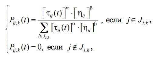
- probability of transition from one vertex to another -
Before you visual work of two algorithms. Once again I will note that a detailed explanation (especially of the ant algorithm) in the comments of the code.
Please note that in imitation annealing, the optimum was already found at 20,000 iterations, then, when the temperature was low enough, the probability of switching to new routes decreased significantly, so the algorithm “got up”. Here you can enter the criteria for stopping. The higher the initial temperature, the greater the likelihood of getting to the optimal route, and the more iterations will be performed, however, it is far from a fact that we will find a global optimum.
In the ant algorithm, everything is different. The main advantage of the ant algorithm is that it will never stop, it will always look for better ways. With an infinite number of iterations (generations), the probability of finding a global optimum will tend to 1. However, at the very beginning the question arose: which initial parameters should we choose? Answer: the method of selection. We are optimizing again. These parameters of the ant optimization were optimized using a genetic algorithm not at these coordinates . There were other coordinates and the number of cities was 50. Not really getting good convergence, I got some parameters that roughly correspond to this example.
On one test, I did not go far, so I bring a table from a series of tests.
One can see the stability of the two algorithms, however, the variation in the mean value of the ant algorithm is smaller.
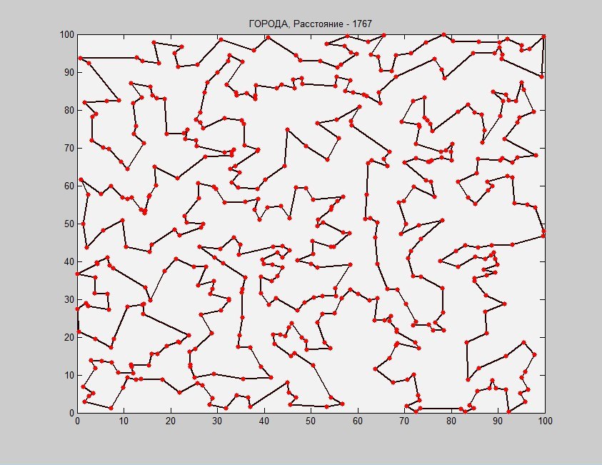
Now let's look at the work of two algorithms per 100 generated cities.
Imitation annealing:
Options:
- The number of cities - 100
- Initial temperature - 42,000
- Final temperature - 0.01
- Temperature formula - initial temperature / kth iteration
- Number of iterations - 420,000
- Acceptance probability function - exp (-ΔE / T)
- Determination of a potential route (generating family) - reversal of a part of a vector (current route) from two randomly selected numbers with a uniform distribution
Now look at the work of the ant algorithm at the same coordinates.
Ant algorithm:
Options:
- Number of iterations (generations) - 50
- Number of ants per generation - 100
- The number of cities - 100
- alpha (coefficient of orientation to pheromones) - 1
- beta (coefficient of orientation to the length of the path) - 3
- e (coefficient evaporation of pheromones) - 0.5
- elite (number of elite ants) - no
- The location of the ants in the first cities is different, without repetition. Number of cities = number of ants in a generation
- pheromone update - global (pheromones are updated after the passage of the 1st generation)
Here the parameters took "by eye".
Again, the ant algorithm showed a better result, however, let's look again at the table from the test series:
Here imitative annealing went far ahead. In general, before I read the article, I was skeptical about imitative annealing. In the development of trading systems (in which I am involved) and their optimization, the annealing method is not suitable, since it is not the local optimum itself that is important for us, but the “spread” around it. On a conditional example: there is a moving average of 15 days on some paper, the yield for the year showed 10,000, and at 14 days (-1000). Here it is important for us that near the optimal parameter the profit should evenly decrease. Therefore, in different situations - different optimization.
As for the traveling salesman task, I, even if not in a “pure” competition (because it didn’t work out the right parameters for the ant algorithm), give up the victory to simulated annealing. If you add a stopping criterion, the same distances can be achieved in 2.5 seconds without much changing the standard deviation, which is not the case with the ant algorithm. According to a series of tests, much of which did not get here, the ant algorithm works brilliantly up to 50 cities, then begins to "drizzle", the optimization time slows down dramatically, which is logical in principle. However, he confidently goes to the global optimum, even if slowly.
Somewhere deep in my heart I still want the ant algorithm to show itself better. Maybe that is why the feeling that I made a mistake somewhere, and not just one, does not leave. Therefore, those who are interested, and those who are just starting their way in this direction - join. Write comments with suggestions, both about the algorithms, and about how best to submit the material.
In the meantime, look at today's winner. 500 cities, 86 seconds of optimization (and this is far from the limit).
Very cool!
Catch up or not the ant algorithm? Will it overtake it genetic? Who will be more effective? About this and another in the following publications.
Useful material:
» Video about ant algorithm (in Russian)
» Video about imitation annealing (in Russian)
» An article about the ant algorithm (in Russian)
» An article about imitation annealing (in Russian)
Source: https://habr.com/ru/post/308960/
All Articles