Computer Science for Postgres Indexes
Friends, PG Day'16 Russia successfully completed, we took a deep breath and are already thinking about how to make upcoming events even more interesting and useful for you. We continue to publish interesting, in our opinion, materials on Postgres and communicate with you in the comments. Today, we present the translation of Pat Shaughnessy’s article on what PostgreSQL indexes are.
We all know that indexes are one of the most powerful and important functions of relational database servers. How to quickly find the value? Create an index. What you need to remember to do when combining two tables? Create an index. How to speed up a SQL query that started to work slowly? Create an index.
But what are these indices? And how do they speed up database searches? To find out, I decided to read the PostgreSQL C database server source code and follow how it searches for an index for a simple text value. I expected to find complex algorithms and efficient data structures. And I found them. Today, I will show you what the indexes look like inside Postgres, and explain how they work.
')
What I did not expect to find — what I first discovered while reading Postgres source code — is the computer science theory at the heart of what it does. Reading the Postgres source code turned into a return to school and the study of the subject for which I never had enough time in my youth. Comments on C inside Postgres explain not only what he does, but why .
When we left the Nautilus team, they were exhausted and almost fainted: the Postgres sequential scanning algorithm thoughtlessly looped through all the entries in the user table! Remember my previous post in which we executed this simple SQL query to find Captain Nemo:
 Postgres processed, analyzed and planned the request. Then ExecSeqScan , function C inside Postgres, which performs the Serially Scan plan node (SEQSCAN), quickly found Captain Nemo:
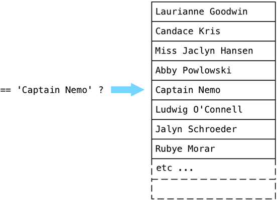
But then Postgres inexplicably continued to perform a cycle across the entire user table, comparing each name with “Captain Nemo”, although we already found what we were looking for!
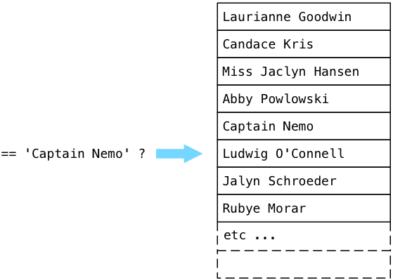
Imagine that there would be millions of records in our table - the process would take a very long time. Of course, we could avoid this by removing the sort and rewriting our query so that only the first found name is accepted, but the deeper problem is the inefficiency of the way Postgres searches our target string. Using sequential scanning to compare each value in the user table with “Captain Nemo” is slow, inefficient and depends on the random order in which the names appear in the table. What are we doing wrong? There must be a better way!
The answer is simple: we forgot to create an index. Let's do it now.
Creating an index is very simple - you just need to run this command:

As Ruby developers, we, of course, would instead use ActiveRecord add_index migration, which will run the same CREATE INDEX command “under the hood”. When we run our select query again, Postgres will, as usual, create a plan tree, but this time it will be slightly different:
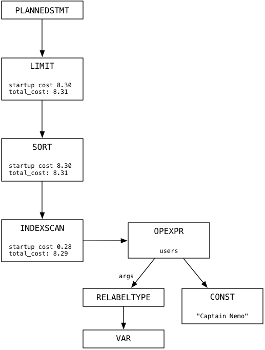
Notice that the bottom Postgres now uses INDEXSCAN instead of SEQSCAN. Unlike SEQSCAN, INDEXSCAN will not scan across the entire user table. Instead, it uses the index that we just created to find and return records about Captain Nemo quickly and efficiently.
Creating an index solved our performance problem, but left us with a lot of interesting unanswered questions:
Let's try to answer these questions by studying the Postgres source code.
We can start by reviewing the documentation for the CREATE INDEX command.
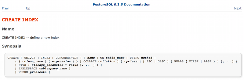
Here you see all the options that we can use to create an index, for example, UNIQUE and CONCURRENTLY. Note that there is an option like the USING method. It tells Postgres what kind of index we need. Below on the same page there is information about the method argument to the keyword USING:

It turns out Postgres implements four different types of indices [approx. Lane: now more, the article was written before BRIN and other new index options appeared.] You can use them for different data types and in different situations. Since we didn’t specify USING, our index_users_on_name is “btree” (or B-Tree) index, the default type.
This is our first clue: the Postgres index is the B-Tree. But what is a B-Tree? Where can we find it? Inside Postgres, of course! Let's look in the source code of the C Postgres files containing “btree:”
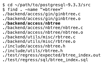
The key result is bold: “./backend/access/nbtree.” Inside this directory is a README file. Let's read it:
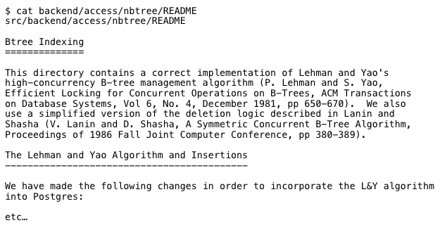 Surprisingly, this README file turned out to be a detailed 12-page document! Postgres source code contains not only useful and interesting comments on code C, but also documentation on the theory and implementation of the database server. Reading and understanding code in open source projects is often difficult and scary, but not in PostgreSQL. The developers behind Postgres have made tremendous efforts so that we can understand their work.
The document title README - “Btree Indexing” - confirms that the directory contains the C code that implements the B-Tree indexes in the Postgrece. But the first sentence is even more interesting: this is a reference to a scientific paper that explains what a B-Tree is and how postgres indexes work: Efficient Locking for Concurrent Operations on B-Trees , authored by Lehman and Yao ).
We will try to deal with the fact that such a B-Tree with the help of this scientific work.
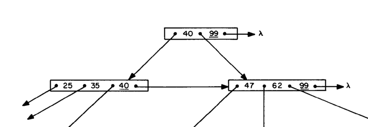
The work of Lehmann and Yao explains the innovative changes they made to the B-Tree algorithm in 1981. Let's talk about it a little later. But they start with a simple introduction to the B-Tree data structure, which was invented 9 years earlier - in 1972. One of their diagrams shows an example of a simple B-Tree:

The term B-Tree is an abbreviation for the English “balanced tree” - a balanced tree. Algorithm makes searching easy and fast. For example, if we wanted to find the value 53 in this example, we would start with the root node containing the value 40:

We compare our sought value 53 with the value we found in the tree node. 53 is more or less than 40? Since 53 is over 40, we follow the pointer down and to the right. If we were looking for 29, we would have gone down to the left. Pointers to the right lead to larger values, and to the left, to smaller ones.
Following down the pointer to the next child node of the tree, we encounter a node containing 2 values:

This time we compare 53 at once with 47 and 62 and find that 47 <53 <62. Note that the values in the tree node are sorted, so it will be easy to do. Now we follow down the central sign.
Here we have another tree node, already with three meanings:
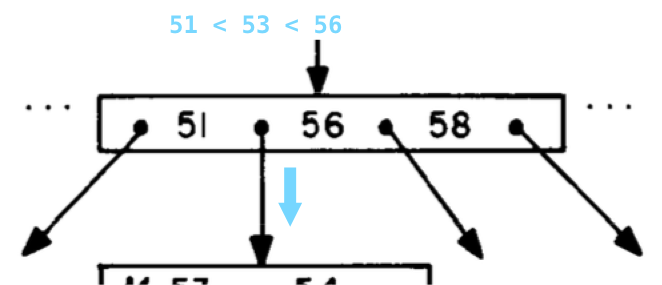
After reviewing the sorted list of numbers, we find 51 <53 <56 and follow down the second of four pointers.
Finally, we arrive at a leaf node of the tree:
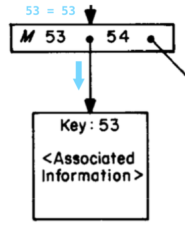
And here it is, our desired value of 53!
The B-Tree algorithm speeds up the search because:
Lehman and Yao drew this diagram over 30 years ago. What does it have to do with how Postgres works today? Amazingly, the index index_users_on_name, which we created earlier, is very similar to this very diagram from scientific work: we created in 2014 an index that looks exactly like a diagram from 1981!
When we ran the CREATE INDEX command, Postgres saved all the names from our user table in B-Tree. They became the keys of the tree. Here is what the node inside the B-Tree index looks like in Postgrese:

Each entry in the index consists of a structure in the C language called IndexTupleData, followed by a bitmap and a value. Postgres uses a bitmap to record if any of the index attributes in the key are NULL, to save space. Actual values are in the index after the bitmap.
Let's take a closer look at the structure of IndexTupleData:
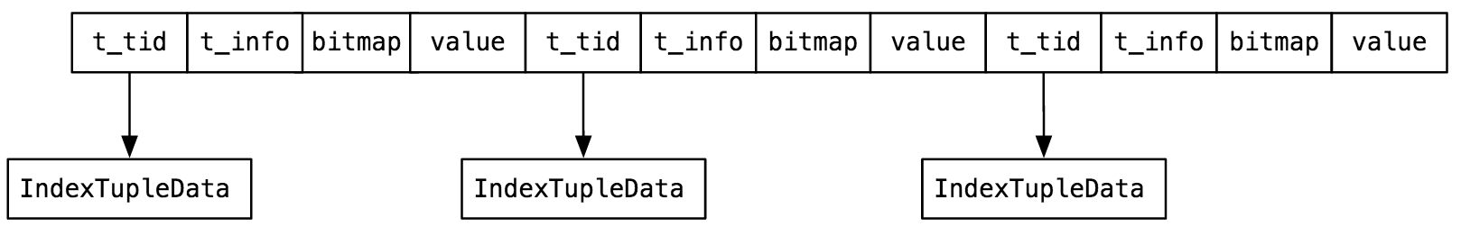
In the figure above, you can see that each IndexTupleData structure contains:
To better understand this, let's show some entries from our index index_users_on_name:
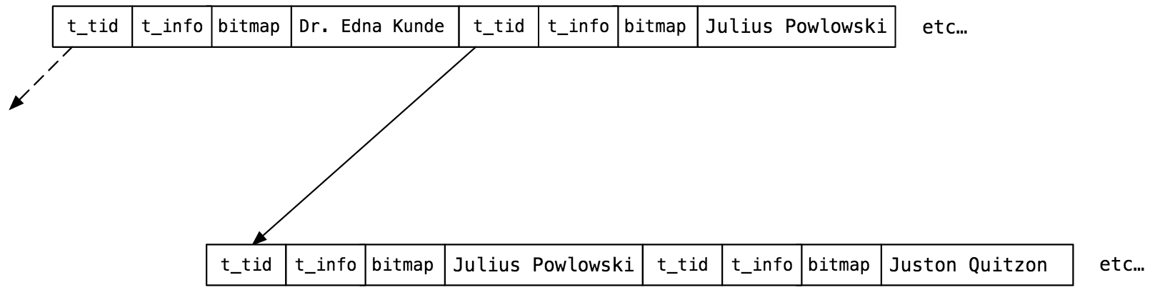
I replaced value with some names from my user table. The top node of the tree contains the keys “Dr. Edna Kunde ”and“ Julius Powlowski ”, and the bottom one is“ Julius Powlowski ”and“ Juston Quitzon ”. Note that unlike the Lehmann and Yao diagrams, Postgres repeats the parent key in each child node. Here “Julius Powlowski” is the key in the top and child nodes. The t_tid pointer in the top node refers to the same name Julius in the bottom node.
To learn more about exactly how Postgres saves key values to a B-Tree node, refer to the itup.h header file:


Let's go back to our original SELECT query:

How exactly does Postgres look for the value “Captain Nemo” in our index index_users_on_name? Why use the index faster than sequential scanning, which we considered in a previous post? To find out, let's zoom out a bit and look at some usernames in our index:
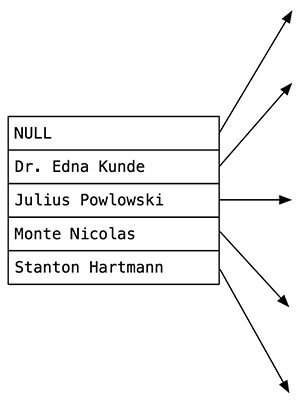
This is the B-Tree root node index_users_on_name. I laid the tree on its side so that the names would fit. You can see 4 names and one NULL value. Postgres created this root node when I created index_users_on_name. Notice that in addition to the first NULL value, which indicates the beginning of the index, the remaining 4 values are more or less evenly distributed in alphabetical order.
Let me remind you that B-Tree is a balanced tree. In this example, there are 5 child nodes in B-Tree:
As we search for the name Captain Nemo, Postgres moves along the first upper arrow to the right. This is because Captain Nemo alphabetically goes before Dr. Edna Kunde:
As you can see, on the right Postgres found the B-Tree node, which contains Captain Nemo. For my test, I added 1000 names to the user table. This child B-Tree node contains about 200 names (240, to be exact). So the B-Tree algorithm significantly narrowed our search to the Postgres.
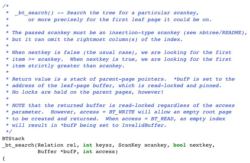
To learn more about the specific algorithm used by Postgres to find the target B-Tree node among all its nodes, read the _bt_search function.
Now that Postgres has narrowed the search space to a B-Tree node containing about 200 names, he still needs to find Captain Nemo among them. How does he do it? Does he apply sequential scanning to this short list?
Not. To search for a key value inside a node of a tree, Postgres switches to using a binary search algorithm. He starts comparing a key located at a 50% position in a tree node with “Captain Nemo”:

Since Captain Nemo alphabetically goes after Breana Witting, Postgres jumps to the 75% position and makes another comparison:

This time Captain Nemo goes to Curtis Wolf, so Postgres comes back a little. After a few more iterations (Postgres took 8 comparisons to find Captain Nemo in my example), Postgres finally finds what we were looking for.
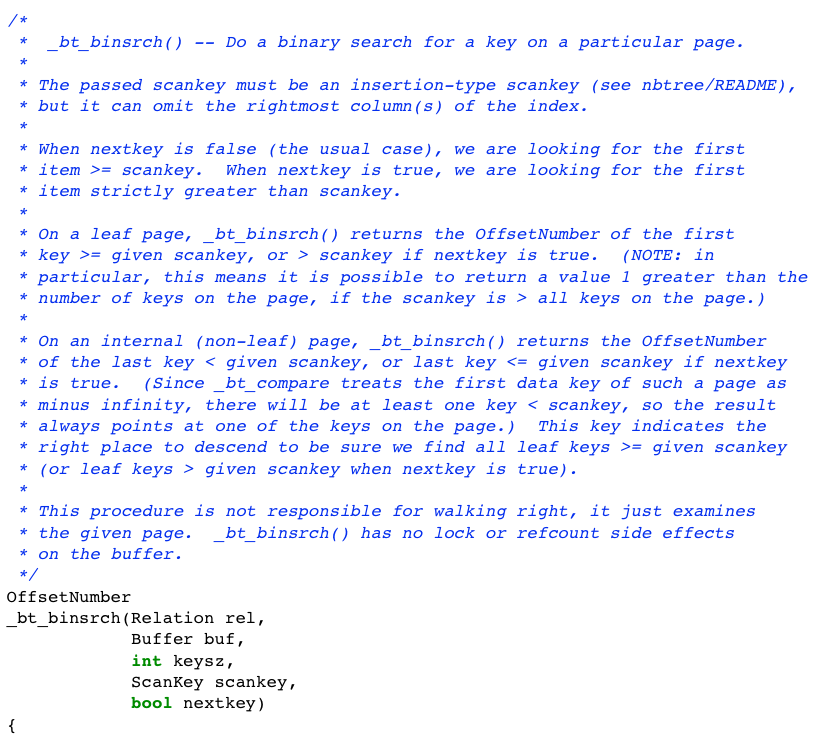
To learn more about how Postgres searches for a value in a particular B-Tree node, read the _bt_binsrch function:
I don’t have enough space in this post to tell about all the exciting details regarding B-Tree, database indexes or Postgres internals ... maybe I should write the Postgres book under a microscope :) In the meantime, here are some interesting theoretical facts that you You can read in Efficient Locking for Concurrent Operations on B-Trees or in other scientific work to which it refers.
Professor Aronnaks risked his life and career to find the elusive Nautilus and join Captain Nemo in a long line of stunning underwater adventures. We should do the same: do not be afraid to dive under the water - deep into the tools, languages and technologies that you use every day. You may know a lot about Postgres, but do you know how it works from the inside? Take a look inside, and do not have time to look back, as you find yourself in an underwater adventure.
Studying at work the computer science behind our applications is not just entertainment, but an important component of the developer development process. Software development tools are improving with each passing year, writing websites and mobile applications is simplified, but we must not lose sight of the fundamental computer science we depend on. We all stand on the shoulders of giants - people like Lehman and Yao, as well as open source developers who used their theories to create a Postgres. Do not take the tools that you use every day for granted - study their device. You will become wiser as a developer and find ideas and knowledge that were not even suspected.
We all know that indexes are one of the most powerful and important functions of relational database servers. How to quickly find the value? Create an index. What you need to remember to do when combining two tables? Create an index. How to speed up a SQL query that started to work slowly? Create an index.
But what are these indices? And how do they speed up database searches? To find out, I decided to read the PostgreSQL C database server source code and follow how it searches for an index for a simple text value. I expected to find complex algorithms and efficient data structures. And I found them. Today, I will show you what the indexes look like inside Postgres, and explain how they work.
')
What I did not expect to find — what I first discovered while reading Postgres source code — is the computer science theory at the heart of what it does. Reading the Postgres source code turned into a return to school and the study of the subject for which I never had enough time in my youth. Comments on C inside Postgres explain not only what he does, but why .
Sequential scan: mindless search
When we left the Nautilus team, they were exhausted and almost fainted: the Postgres sequential scanning algorithm thoughtlessly looped through all the entries in the user table! Remember my previous post in which we executed this simple SQL query to find Captain Nemo:
But then Postgres inexplicably continued to perform a cycle across the entire user table, comparing each name with “Captain Nemo”, although we already found what we were looking for!
Imagine that there would be millions of records in our table - the process would take a very long time. Of course, we could avoid this by removing the sort and rewriting our query so that only the first found name is accepted, but the deeper problem is the inefficiency of the way Postgres searches our target string. Using sequential scanning to compare each value in the user table with “Captain Nemo” is slow, inefficient and depends on the random order in which the names appear in the table. What are we doing wrong? There must be a better way!
The answer is simple: we forgot to create an index. Let's do it now.
Create index
Creating an index is very simple - you just need to run this command:
As Ruby developers, we, of course, would instead use ActiveRecord add_index migration, which will run the same CREATE INDEX command “under the hood”. When we run our select query again, Postgres will, as usual, create a plan tree, but this time it will be slightly different:
Notice that the bottom Postgres now uses INDEXSCAN instead of SEQSCAN. Unlike SEQSCAN, INDEXSCAN will not scan across the entire user table. Instead, it uses the index that we just created to find and return records about Captain Nemo quickly and efficiently.
Creating an index solved our performance problem, but left us with a lot of interesting unanswered questions:
- What exactly is the postgrese index?
- If I could get into the Postgres database and get a better look at the index, what would it look like ?
- How does the index speed up the search?
Let's try to answer these questions by studying the Postgres source code.
What is the postgres index?
We can start by reviewing the documentation for the CREATE INDEX command.
Here you see all the options that we can use to create an index, for example, UNIQUE and CONCURRENTLY. Note that there is an option like the USING method. It tells Postgres what kind of index we need. Below on the same page there is information about the method argument to the keyword USING:
It turns out Postgres implements four different types of indices [approx. Lane: now more, the article was written before BRIN and other new index options appeared.] You can use them for different data types and in different situations. Since we didn’t specify USING, our index_users_on_name is “btree” (or B-Tree) index, the default type.
This is our first clue: the Postgres index is the B-Tree. But what is a B-Tree? Where can we find it? Inside Postgres, of course! Let's look in the source code of the C Postgres files containing “btree:”
The key result is bold: “./backend/access/nbtree.” Inside this directory is a README file. Let's read it:
The document title README - “Btree Indexing” - confirms that the directory contains the C code that implements the B-Tree indexes in the Postgrece. But the first sentence is even more interesting: this is a reference to a scientific paper that explains what a B-Tree is and how postgres indexes work: Efficient Locking for Concurrent Operations on B-Trees , authored by Lehman and Yao ).
We will try to deal with the fact that such a B-Tree with the help of this scientific work.
What does the B-Tree index look like?
The work of Lehmann and Yao explains the innovative changes they made to the B-Tree algorithm in 1981. Let's talk about it a little later. But they start with a simple introduction to the B-Tree data structure, which was invented 9 years earlier - in 1972. One of their diagrams shows an example of a simple B-Tree:
The term B-Tree is an abbreviation for the English “balanced tree” - a balanced tree. Algorithm makes searching easy and fast. For example, if we wanted to find the value 53 in this example, we would start with the root node containing the value 40:
We compare our sought value 53 with the value we found in the tree node. 53 is more or less than 40? Since 53 is over 40, we follow the pointer down and to the right. If we were looking for 29, we would have gone down to the left. Pointers to the right lead to larger values, and to the left, to smaller ones.
Following down the pointer to the next child node of the tree, we encounter a node containing 2 values:
This time we compare 53 at once with 47 and 62 and find that 47 <53 <62. Note that the values in the tree node are sorted, so it will be easy to do. Now we follow down the central sign.
Here we have another tree node, already with three meanings:
After reviewing the sorted list of numbers, we find 51 <53 <56 and follow down the second of four pointers.
Finally, we arrive at a leaf node of the tree:
And here it is, our desired value of 53!
The B-Tree algorithm speeds up the search because:
- it sorts values (called keys) within each node;
- it is balanced: the keys are equally distributed between the nodes, minimizing the number of transitions from one node to another. Each pointer leads to a child node, which contains approximately the same number of keys as each subsequent child node.
What does the postgres index look like?
Lehman and Yao drew this diagram over 30 years ago. What does it have to do with how Postgres works today? Amazingly, the index index_users_on_name, which we created earlier, is very similar to this very diagram from scientific work: we created in 2014 an index that looks exactly like a diagram from 1981!
When we ran the CREATE INDEX command, Postgres saved all the names from our user table in B-Tree. They became the keys of the tree. Here is what the node inside the B-Tree index looks like in Postgrese:
Each entry in the index consists of a structure in the C language called IndexTupleData, followed by a bitmap and a value. Postgres uses a bitmap to record if any of the index attributes in the key are NULL, to save space. Actual values are in the index after the bitmap.
Let's take a closer look at the structure of IndexTupleData:
In the figure above, you can see that each IndexTupleData structure contains:
- t_tid: this is a pointer to either another index tuple or a record in the database. Notice that this is not a pointer to physical memory in the C language. Instead, it contains numbers that Postgres can use to find the desired value on the memory pages.
- t_info: it contains information about the elements of the index, for example, how many values there are and whether they are equal to null.
To better understand this, let's show some entries from our index index_users_on_name:
I replaced value with some names from my user table. The top node of the tree contains the keys “Dr. Edna Kunde ”and“ Julius Powlowski ”, and the bottom one is“ Julius Powlowski ”and“ Juston Quitzon ”. Note that unlike the Lehmann and Yao diagrams, Postgres repeats the parent key in each child node. Here “Julius Powlowski” is the key in the top and child nodes. The t_tid pointer in the top node refers to the same name Julius in the bottom node.
To learn more about exactly how Postgres saves key values to a B-Tree node, refer to the itup.h header file:
IndexTupleData
view on postgresql.orgSearch for a B-Tree node containing Captain Nemo
Let's go back to our original SELECT query:
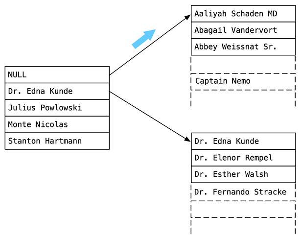
How exactly does Postgres look for the value “Captain Nemo” in our index index_users_on_name? Why use the index faster than sequential scanning, which we considered in a previous post? To find out, let's zoom out a bit and look at some usernames in our index:
This is the B-Tree root node index_users_on_name. I laid the tree on its side so that the names would fit. You can see 4 names and one NULL value. Postgres created this root node when I created index_users_on_name. Notice that in addition to the first NULL value, which indicates the beginning of the index, the remaining 4 values are more or less evenly distributed in alphabetical order.
Let me remind you that B-Tree is a balanced tree. In this example, there are 5 child nodes in B-Tree:
- alphabetical names before Dr. Edna Kunde;
- names located between Dr. Edna Kunde and Julius Powlowski;
- names located between Julius Powlowski and Monte Nicolas;
- etc.
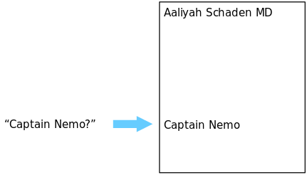
As we search for the name Captain Nemo, Postgres moves along the first upper arrow to the right. This is because Captain Nemo alphabetically goes before Dr. Edna Kunde:
As you can see, on the right Postgres found the B-Tree node, which contains Captain Nemo. For my test, I added 1000 names to the user table. This child B-Tree node contains about 200 names (240, to be exact). So the B-Tree algorithm significantly narrowed our search to the Postgres.
To learn more about the specific algorithm used by Postgres to find the target B-Tree node among all its nodes, read the _bt_search function.
_bt_search
view on postgresql.orgSearch for Captain Nemo inside a specific B-Tree site
Now that Postgres has narrowed the search space to a B-Tree node containing about 200 names, he still needs to find Captain Nemo among them. How does he do it? Does he apply sequential scanning to this short list?
Not. To search for a key value inside a node of a tree, Postgres switches to using a binary search algorithm. He starts comparing a key located at a 50% position in a tree node with “Captain Nemo”:
Since Captain Nemo alphabetically goes after Breana Witting, Postgres jumps to the 75% position and makes another comparison:
This time Captain Nemo goes to Curtis Wolf, so Postgres comes back a little. After a few more iterations (Postgres took 8 comparisons to find Captain Nemo in my example), Postgres finally finds what we were looking for.
To learn more about how Postgres searches for a value in a particular B-Tree node, read the _bt_binsrch function:
_bt_binsrch
view on postgresql.orgThere is still much to learn
I don’t have enough space in this post to tell about all the exciting details regarding B-Tree, database indexes or Postgres internals ... maybe I should write the Postgres book under a microscope :) In the meantime, here are some interesting theoretical facts that you You can read in Efficient Locking for Concurrent Operations on B-Trees or in other scientific work to which it refers.
- Inserts in B-Tree: The most beautiful part of the B-Tree algorithm is adding new keys to the tree. They are added in sorted order to the appropriate tree node, but what happens when there is no room for new keys? In this case, Postgres divides the node into two, inserts a new key into one of them, and adds the key from the divided node to the parent node along with a pointer to the new child node. Of course, there is a possibility that the parent node will also have to be split in order to add a new key, which will lead to a complex recursive operation.
- Deleting from B-Tree: the reverse operation is also interesting. When a key is removed from a node, Postgres merges sibling nodes, if possible, by removing the key from their parent node. This operation can also be recursive.
- B-Link- Tree: The work of Lehman and Yao talks about the innovation that they explored in relation to concurrency and blocking, when several threads use the same B-Tree. As you remember, the Postgres code and algorithms must be multi-threaded, because many clients can search and modify the same index at the same time. Adding another pointer from each B-Tree node to the next child node, the so-called “right arrow”, can search one thread in the tree, even if the second thread divides the nodes without blocking the entire index:
Do not be afraid to explore the invisible part of the iceberg
Professor Aronnaks risked his life and career to find the elusive Nautilus and join Captain Nemo in a long line of stunning underwater adventures. We should do the same: do not be afraid to dive under the water - deep into the tools, languages and technologies that you use every day. You may know a lot about Postgres, but do you know how it works from the inside? Take a look inside, and do not have time to look back, as you find yourself in an underwater adventure.
Studying at work the computer science behind our applications is not just entertainment, but an important component of the developer development process. Software development tools are improving with each passing year, writing websites and mobile applications is simplified, but we must not lose sight of the fundamental computer science we depend on. We all stand on the shoulders of giants - people like Lehman and Yao, as well as open source developers who used their theories to create a Postgres. Do not take the tools that you use every day for granted - study their device. You will become wiser as a developer and find ideas and knowledge that were not even suspected.
Source: https://habr.com/ru/post/308752/
All Articles