OpenCV and image processing
Good morning, ladies and gentlemen. Attentive readers noticed that translated books on the topic of computer vision had once again appeared on the Russian market. We also could not but be interested in the following book:
Since computer vision technologies are largely tied to both Python and C ++, we picked up an article with task analysis and code in both languages. In addition, we sincerely hope that you will like the girl under the cut.
This article will explain how to generate averaged face image using the OpenCV library (C ++ / Python).
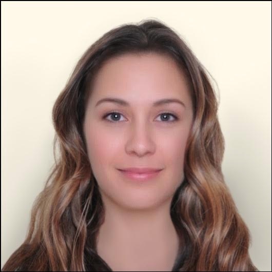
Fig. one
')
The woman shown in Fig. 1, most readers will find it pretty. But can you guess her nationality? Why does she have such a smooth skin? That's right - this woman does not exist. But you can not say that this is a completely virtual image. This is the average portrait of all employees of my company Sight Commerce Inc. as of about 2011. Her nationality is difficult to determine, since we have girls with European, Latin American, East Asian and Indian roots!
The history of averaging faces is just fascinating.
It all started with the research of Francis Galton (cousin Charles Darwin), who in 1878 invented a new photographic technique: he learned how to combine faces and make the first identikits. He believed that by combining the faces of criminals, one could model the “prototypical” face of a felon and subsequently recognize potential criminals by their features. It turned out that this hypothesis is erroneous: after examining someone else's photo, it is impossible to determine his tendency to crimes.
However, Galton noticed that the average face always looks more attractive than all the "components" of his faces. In one striking experiment, the researchers "laid down" the faces of all 22 finalists of the Miss Germany 2002 contest. The respondents rated the resulting portrait higher than any of the contestants, even higher than “Miss Berlin”, which then turned out to be the winner. Phew! It turns out that Jessica Alba is so pretty precisely because her face is close to the average.
Is it possible to equate "average" to "mediocre"? Why does the average face seem attractive to us? According to an evolutionary hypothesis called “coinophilia,” individuals in active reproductive age are looking for partners with averaged features, since deviations from the mean may indicate harmful mutations. In addition, the middle face is symmetrical, since the variations in the left and right sides of the face are mutually smoothed out.
How to generate averaged face in OpenCV?
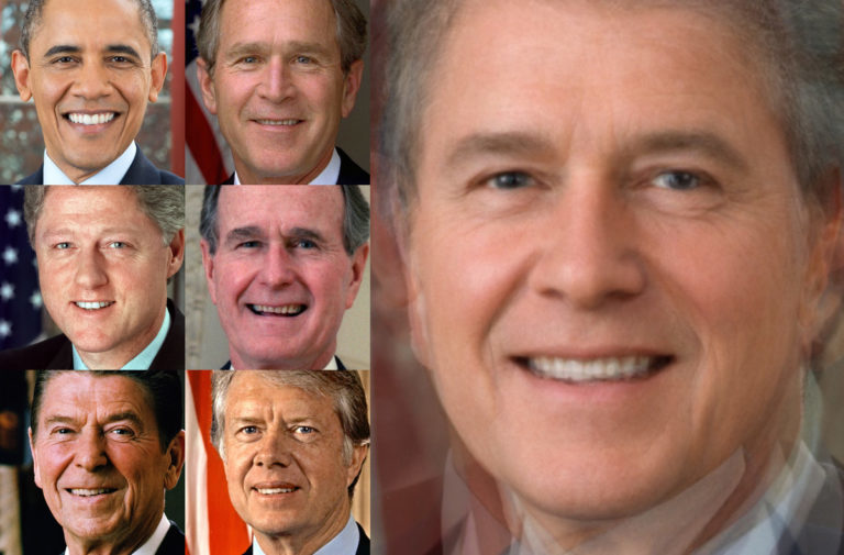
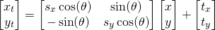
Fig. 2: The average face of US presidents from Carter to Obama
The code and images for the article can be downloaded here .
The following is a step-by-step description of how to generate an average face, having the above set of images. In this case, we do not take into account the size of the images themselves or the size of the face on each portrait.
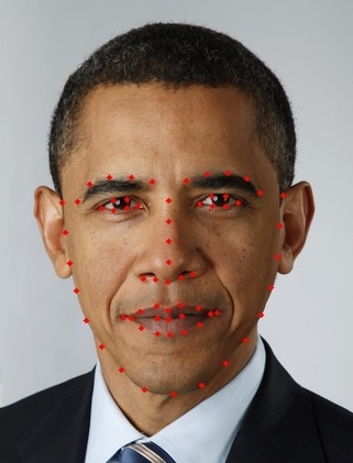
Fig. 3: Facial feature detection example
For each portrait, we calculate 68 “control points” using the dlib library. How to install and use dlib, I tell in detail in another post Facial Feature Detection . The portrait of Obama has 68 control points.
At the entrance, the size of face images can be very different. Therefore, we will have to normalize them and lead to a single reference system. To do this, we deform all face images to size 600 × 600 so that the left corner of the left eye is at the point with coordinates (180, 200), and the right corner of the right eye is at the point (420, 200). Let's call this reference system the “final coordinate system,” and the coordinates of the original images, the “initial coordinate system . ”
How do I choose the points above? I wanted to ensure that these points would be located on the same horizontal line, and this line would run approximately a third of the way from the top to the bottom edge of the picture. So, I ensured that the tips of the sockets were located at points with coordinates (0.3 x width, height / 3) and (0.7 x width, height / 3).
We also know where the corners of the eyes are on the source images, respectively, at control points 36 and 45. Then we can calculate the similarity transformation (rotation, translation, scaling) and translate the points from the initial coordinate system to the final one.
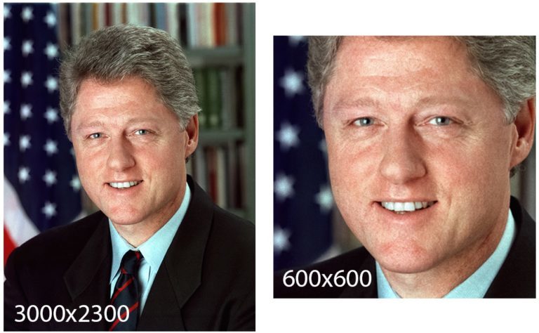
Fig. 4: Similarity conversion is used to transform an original 3000 × 2300 image into a final image of 600 × 600.
What is similarity conversion? The similarity transformation is a 2 × 3 matrix that allows you to change the location of the points (x, y) or the whole image. The first two columns of this matrix encode rotation and scaling, and the last one is the translation (i.e. offset). Suppose you transform (move) the four corners of a square in such a way that the square is scaled in the x and y directions s x and s y times, respectively. At the same time, it rotates through an angle θ and is transferred (moved) by t x and t y in the x and y directions. The similarity transformation can be written as follows:
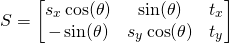
Based on the point (x, y), the similarity transformation described above transfers this point to (x t , y t ) according to the following equation:
Similarity transformation can be performed using
However, there is one small problem. OpenCV requires that you specify at least three pairs of points. This is stupid, since the similarity transformation can be done with just two points. Therefore, you can simply imagine the third point, so that it and the two known points form an equilateral triangle. Then use the
By calculating the similarity transformation, you can use it to transform the original image and its control points into final coordinates. The image is transformed with
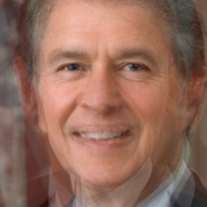
Fig. 5: Simplified face averaging result
At the previous stage, we were able to convert all the images and control points to the coordinates of the final image. Now all our images are the same size, the corners of the eyes are aligned. Perhaps it would be tempting to try to get an average image by taking the average pixel values of these aligned images. However, in this case, you get such a picture, as in Fig. 5. Yes, eyes are aligned, and all other facial features are located at random.
If we knew which point from one source image corresponded to which point from another source image, we could ideally superimpose two images on each other. But we have no such information. We only know the position of the 68 corresponding points on each of the original images. Focusing on these points, we will divide each image into triangular areas, and first we will align these areas, and then we will average pixel values.
This process is described in more detail in my post Face Morphing , and in general terms - below.
Calculate the average front points
To calculate how the average face will look, all the features of which are aligned, first you need to calculate the average of all the converted control points in the final image. To do this, we simply average the x and y values of all control points in the coordinates of the final image.
Delaunay Triangulation Calculation
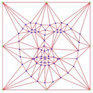
Fig. 6: Calculation of the Delaunay triangulation for the average control points.
At the previous stage, we obtained the positions of the control points for the average face in the final coordinates. You can use these 68 points (shown in blue in Figure 6) and 8 points on the border of the final image (shown in green) to calculate the Delaunay triangulation (shown in red). More details Delone triangulation is described here .
Delaunay triangulation allows you to split the image into triangles. As a result of this triangulation, we obtain a list of triangles represented as an array of indices of 76 points (68 points on the face + 8 boundary points). In the triangulation example shown below, it is noticeable that the control points 62, 68 and 60 form a triangle, 32, 50 and 49 form another triangle, etc.
Deformation of triangles
Triangulation example
At the previous stage, we calculated the average location of control points on the face and, based on this data, performed the Delaunay triangulation to divide the image into triangles. In fig. 7 we can see the Delone triangles superimposed on the transformed original image, and on the image that is in the middle, the triangulation of the averaged control points is shown. Note that triangle 1 in the image on the left corresponds to triangle 1 in the middle image. Knowing the three vertices of the triangle 1 located on the left image and the corresponding three vertices of the triangle from the middle image, we can calculate the affine transformation. Repeating this procedure for each of the triangles from the left image, we get the right image. So, the right image is the result of the deformation of the left to the state of the averaged face.

Fig. 7: Deformation of the image based on the Delaunay triangulation
Applying the manipulations from the previous stage to all the source images, we obtain the final images, which are deformed in such a way that the result coincides with the averaged end points. To calculate the average image, you can simply add the pixel intensity values of all the deformed images and divide this amount by the number of images. In fig. 2 shows the result of such averaging. It looks much better than the “average” that was in fig. five.
What do you think the “average” US president looks like? In my opinion - fatherly and cute.
Face averaging results
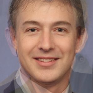
Fig. 8: The average face of Mark Zuckerberg, Larry Page, Ilona Mask and Jeff Bezos
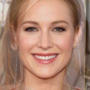
Fig. 9: Average face of Bree Larson, Julianne Moore, Cate Blanchett and Jennifer Lawrence
What is the average leading entrepreneur technician? In fig. Figure 8 shows the average face of Mark Zuckerberg, Larry Page, Ilon Mask and Jeff Bezos. I can not say about this "average entrepreneur" anything special except that he still can see the hair (despite the negative contribution of Jeff Bezos).
What is the average Oscar-winning actress? In fig. Figure 9 shows the average face of Bree Larson, Julianne Moore, Cate Blanchett and Jennifer Lawrence. So, the average movie star is very pretty. And her teeth are better than those of a successful entrepreneur. No wonder.
You can also make a symmetrical face by averaging it with a mirror image. An example is shown below.
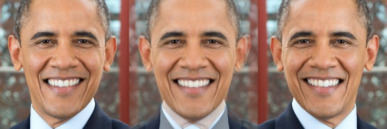
Fig. 10: Symmetrical President Obama (center) obtained by averaging his photo (left) with his own mirror image (right).
Since computer vision technologies are largely tied to both Python and C ++, we picked up an article with task analysis and code in both languages. In addition, we sincerely hope that you will like the girl under the cut.
This article will explain how to generate averaged face image using the OpenCV library (C ++ / Python).
Fig. one
')
The woman shown in Fig. 1, most readers will find it pretty. But can you guess her nationality? Why does she have such a smooth skin? That's right - this woman does not exist. But you can not say that this is a completely virtual image. This is the average portrait of all employees of my company Sight Commerce Inc. as of about 2011. Her nationality is difficult to determine, since we have girls with European, Latin American, East Asian and Indian roots!
The history of averaging faces is just fascinating.
It all started with the research of Francis Galton (cousin Charles Darwin), who in 1878 invented a new photographic technique: he learned how to combine faces and make the first identikits. He believed that by combining the faces of criminals, one could model the “prototypical” face of a felon and subsequently recognize potential criminals by their features. It turned out that this hypothesis is erroneous: after examining someone else's photo, it is impossible to determine his tendency to crimes.
However, Galton noticed that the average face always looks more attractive than all the "components" of his faces. In one striking experiment, the researchers "laid down" the faces of all 22 finalists of the Miss Germany 2002 contest. The respondents rated the resulting portrait higher than any of the contestants, even higher than “Miss Berlin”, which then turned out to be the winner. Phew! It turns out that Jessica Alba is so pretty precisely because her face is close to the average.
Is it possible to equate "average" to "mediocre"? Why does the average face seem attractive to us? According to an evolutionary hypothesis called “coinophilia,” individuals in active reproductive age are looking for partners with averaged features, since deviations from the mean may indicate harmful mutations. In addition, the middle face is symmetrical, since the variations in the left and right sides of the face are mutually smoothed out.
How to generate averaged face in OpenCV?
Fig. 2: The average face of US presidents from Carter to Obama
The code and images for the article can be downloaded here .
The following is a step-by-step description of how to generate an average face, having the above set of images. In this case, we do not take into account the size of the images themselves or the size of the face on each portrait.
Stage 1: Detection of facial features
Fig. 3: Facial feature detection example
For each portrait, we calculate 68 “control points” using the dlib library. How to install and use dlib, I tell in detail in another post Facial Feature Detection . The portrait of Obama has 68 control points.
Stage 2: Coordinate Transformation
At the entrance, the size of face images can be very different. Therefore, we will have to normalize them and lead to a single reference system. To do this, we deform all face images to size 600 × 600 so that the left corner of the left eye is at the point with coordinates (180, 200), and the right corner of the right eye is at the point (420, 200). Let's call this reference system the “final coordinate system,” and the coordinates of the original images, the “initial coordinate system . ”
How do I choose the points above? I wanted to ensure that these points would be located on the same horizontal line, and this line would run approximately a third of the way from the top to the bottom edge of the picture. So, I ensured that the tips of the sockets were located at points with coordinates (0.3 x width, height / 3) and (0.7 x width, height / 3).
We also know where the corners of the eyes are on the source images, respectively, at control points 36 and 45. Then we can calculate the similarity transformation (rotation, translation, scaling) and translate the points from the initial coordinate system to the final one.
Fig. 4: Similarity conversion is used to transform an original 3000 × 2300 image into a final image of 600 × 600.
What is similarity conversion? The similarity transformation is a 2 × 3 matrix that allows you to change the location of the points (x, y) or the whole image. The first two columns of this matrix encode rotation and scaling, and the last one is the translation (i.e. offset). Suppose you transform (move) the four corners of a square in such a way that the square is scaled in the x and y directions s x and s y times, respectively. At the same time, it rotates through an angle θ and is transferred (moved) by t x and t y in the x and y directions. The similarity transformation can be written as follows:
Based on the point (x, y), the similarity transformation described above transfers this point to (x t , y t ) according to the following equation:
Similarity transformation can be performed using
estimateRigidTransform // C++ // inPts outPts – , // , , // cv::estimateRigidTransform(inPts, outPts, false); # Python # inPts outPts - numpy # , , # cv2.estimateRigidTransform(inPts, outPts, False); However, there is one small problem. OpenCV requires that you specify at least three pairs of points. This is stupid, since the similarity transformation can be done with just two points. Therefore, you can simply imagine the third point, so that it and the two known points form an equilateral triangle. Then use the
estimateRigidTransform as if we have three pairs of points.By calculating the similarity transformation, you can use it to transform the original image and its control points into final coordinates. The image is transformed with
warpAffine , and the points with the help of transform .Stage 3: Face Alignment
Fig. 5: Simplified face averaging result
At the previous stage, we were able to convert all the images and control points to the coordinates of the final image. Now all our images are the same size, the corners of the eyes are aligned. Perhaps it would be tempting to try to get an average image by taking the average pixel values of these aligned images. However, in this case, you get such a picture, as in Fig. 5. Yes, eyes are aligned, and all other facial features are located at random.
If we knew which point from one source image corresponded to which point from another source image, we could ideally superimpose two images on each other. But we have no such information. We only know the position of the 68 corresponding points on each of the original images. Focusing on these points, we will divide each image into triangular areas, and first we will align these areas, and then we will average pixel values.
This process is described in more detail in my post Face Morphing , and in general terms - below.
Calculate the average front points
To calculate how the average face will look, all the features of which are aligned, first you need to calculate the average of all the converted control points in the final image. To do this, we simply average the x and y values of all control points in the coordinates of the final image.
Delaunay Triangulation Calculation
Fig. 6: Calculation of the Delaunay triangulation for the average control points.
At the previous stage, we obtained the positions of the control points for the average face in the final coordinates. You can use these 68 points (shown in blue in Figure 6) and 8 points on the border of the final image (shown in green) to calculate the Delaunay triangulation (shown in red). More details Delone triangulation is described here .
Delaunay triangulation allows you to split the image into triangles. As a result of this triangulation, we obtain a list of triangles represented as an array of indices of 76 points (68 points on the face + 8 boundary points). In the triangulation example shown below, it is noticeable that the control points 62, 68 and 60 form a triangle, 32, 50 and 49 form another triangle, etc.
Deformation of triangles
Triangulation example
[ 62 68 60 32 50 49 15 16 72 9 8 58 53 35 36 … ] At the previous stage, we calculated the average location of control points on the face and, based on this data, performed the Delaunay triangulation to divide the image into triangles. In fig. 7 we can see the Delone triangles superimposed on the transformed original image, and on the image that is in the middle, the triangulation of the averaged control points is shown. Note that triangle 1 in the image on the left corresponds to triangle 1 in the middle image. Knowing the three vertices of the triangle 1 located on the left image and the corresponding three vertices of the triangle from the middle image, we can calculate the affine transformation. Repeating this procedure for each of the triangles from the left image, we get the right image. So, the right image is the result of the deformation of the left to the state of the averaged face.
Fig. 7: Deformation of the image based on the Delaunay triangulation
Stage 4: Facial Averaging
Applying the manipulations from the previous stage to all the source images, we obtain the final images, which are deformed in such a way that the result coincides with the averaged end points. To calculate the average image, you can simply add the pixel intensity values of all the deformed images and divide this amount by the number of images. In fig. 2 shows the result of such averaging. It looks much better than the “average” that was in fig. five.
What do you think the “average” US president looks like? In my opinion - fatherly and cute.
Face averaging results
Fig. 8: The average face of Mark Zuckerberg, Larry Page, Ilona Mask and Jeff Bezos
Fig. 9: Average face of Bree Larson, Julianne Moore, Cate Blanchett and Jennifer Lawrence
What is the average leading entrepreneur technician? In fig. Figure 8 shows the average face of Mark Zuckerberg, Larry Page, Ilon Mask and Jeff Bezos. I can not say about this "average entrepreneur" anything special except that he still can see the hair (despite the negative contribution of Jeff Bezos).
What is the average Oscar-winning actress? In fig. Figure 9 shows the average face of Bree Larson, Julianne Moore, Cate Blanchett and Jennifer Lawrence. So, the average movie star is very pretty. And her teeth are better than those of a successful entrepreneur. No wonder.
You can also make a symmetrical face by averaging it with a mirror image. An example is shown below.
Fig. 10: Symmetrical President Obama (center) obtained by averaging his photo (left) with his own mirror image (right).
Source: https://habr.com/ru/post/308720/
All Articles