In the shadow of a random forest

1. Introduction

This is a short story about the practical issues of machine learning for large-scale statistical studies of various data on the Internet. The topic of applying basic methods of mathematical statistics for data analysis will also be discussed.

2. Classification by the assessor

The assessor often encounters normally distributed data sets. There is a rule according to which, under a normal distribution (it is called a Gaussian distribution), the random variable rarely deviates by more than three sigmas (the Greek letter “sigma” denotes the square root of the variance, that is, the standard deviation) from its expected value. In other words: in a normal distribution, most objects will differ little from the average. Consequently, the histogram will be as follows:

Such a random variable can correlate with another quantity and even form groups (clusters) according to some signs of similarity. Consider a small example. Assume that we have information about the mass and height of the object, and also know that in the general population there are objects of only two classes (bicycle and truck). Obviously, the height and weight of the truck is clearly greater than that of a bicycle, therefore, both indicators are incredibly valuable for classification.

If we display a cloud of points in two-dimensional space, the coordinates of which are given by the studied pair of sets, then it will be obvious that the points are not distributed randomly, but are grouped into groups (clusters). Consequently, the space can be divided into a linear (hyperplane), which will allow to distinguish trucks from bicycles (for example, if the mass is more than 1000 kg, then this is clearly a truck).

Moreover, it is possible to fix a linear relationship between these metrics (with increasing position along the ordinate there is a clear increase on the abscissa). Thus, the dots line up from the lower left corner to the upper right corner, as if around a stretched thread. For greater clarity, we will add (by the least squares method) a straight line of regression analysis, note the centroids of the clusters, and also display the graphs of these variables:

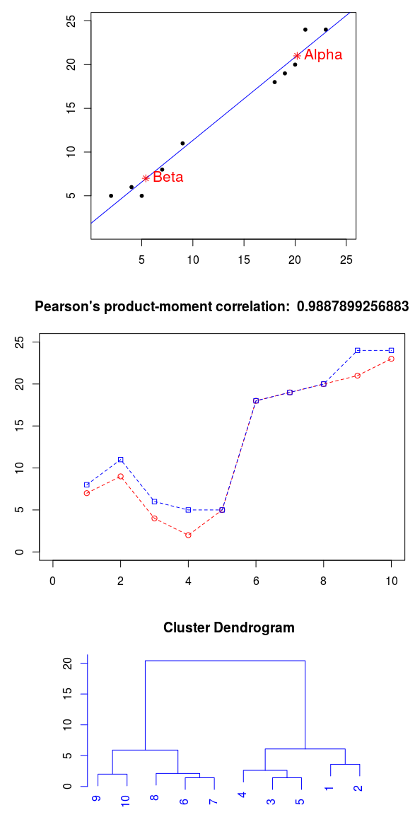
Using the available data, we calculate the degree of relationship. For such datasets in mathematical statistics, the linear correlation coefficient of Karl Pearson is used. This is quite convenient, since it is in the range from -1 to 1. To calculate it, it is necessary to divide the covariance by the product of the standard deviations of the sets (the square root of the variance). By the way, the covariance does not change, if we swap the compared sets, and if they are the same, we get the variance of the random variable. It is important to note that the relationship must be strictly linear.

However, there are a number of other independent variables (predictors) that influence the dependent (criterial) variable. There is no functional dependence, which would allow to calculate one variable by the formula, knowing the other. For example, this is how a person's height depends on weight (dependence exists, but there is no formula that allows knowing only weight to accurately calculate height). How to act if there are a lot of variables and it is necessary to evaluate the importance of each of them?

One approach to solving this problem is the use of machine learning algorithms. For example, the CART algorithm (developed by the scientists Leo Breiman, Jerome Friedman, Charles Stone and Richard Olschen in the early 80s of the 20th century) will make it possible to display decision trees quite well. Naturally, he assumes that all the vectors of features are already labeled by the assessor. However, for more complex tasks, Random forest or Gradient Boosting is more often used. Using the methods mentioned (as well as logistic regression), we visually reflect the degree of importance of each variable:

Naturally, the choice of methods directly depends on the task and the specifics of the data set. But in the vast majority of tasks, automatic classification begins with a preliminary data analysis. It is likely that assessors and experts will be able to see important patterns simply by studying the visual presentation of data and indicators of descriptive statistics (correlation, minimum value, maximum value, average value, median, quartile, variance).

3. Automatic classification

In fact, instead of a specific object (site, person, car, plane), we are faced with a set of its characteristics (mass, speed, presence of USB). This means that the process of turning an entity into a feature vector occurs. So how to deal with really complex data sets?

A single approach cannot exist, since there are so many specific requirements. For automatic image recognition, some algorithms are needed (for example, artificial neural networks), and for complex linguistic text analysis, completely different ones are needed.

In the overwhelming majority of cases, machine learning begins with pre-clearing data. At this stage, the removal of obviously unsuitable objects and simpler methods of classification may occur. The following example searches for centroids of two clusters. A rather popular solution (the recently published second version of Apache Spark) will be a concrete implementation.

import org.apache.spark.mllib.clustering.{KMeans, KMeansModel} import org.apache.spark.mllib.linalg.Vectors val data = sc.textFile(clusterDataFile).map(s => Vectors.dense(s.split(',').map(_.toDouble))).cache() KMeans.train(data, 2, 100).clusterCenters.map(h => h(0) + "," + h(1)).mkString("\n") 

As the complexity of the task increases, so does the complexity of machine learning systems. For example, some search engines use the Gradient Boosting Machine to automatically analyze the quality of sites. Such an algorithm builds a large number of decision trees that use boosting (gradual improvement through improving the prediction quality of previous decision trees). Let's move on to an example. Here are a few lines from the input file:

 0 1:86 2:33 3:79 4:77 5:74 6:81 7:90 8:63 9:8 10:27 11:33 12:29 13:99 14:14 15:92 1 1:100 2:82 3:18 4:8 5:73 6:27 7:18 8:11 9:25 10:46 11:79 12:88 13:62 14:12 15:20 0 1:98 2:53 3:79 4:74 5:26 6:60 7:64 8:89 9:67 10:91 11:22 12:95 13:90 14:35 15:87 0 1:89 2:17 3:4 4:96 5:89 6:31 7:13 8:99 9:55 10:59 11:78 12:43 13:20 14:90 15:62 0 1:20 2:88 3:14 4:99 5:62 6:40 7:58 8:26 9:28 10:25 11:16 12:49 13:20 14:5 15:84 0 1:6 2:94 3:100 4:10 5:89 6:88 7:40 8:2 9:87 10:95 11:61 12:65 13:37 14:81 15:55 1 1:99 2:100 3:42 4:12 5:98 6:4 7:52 8:56 9:29 10:79 11:80 12:44 13:28 14:99 15:49 0 1:5 2:42 3:11 4:14 5:31 6:98 7:54 8:33 9:85 10:48 11:93 12:49 13:85 14:73 15:3 

Suppose that this is some statistics on the most important behavioral factors. The first character of the string is the class (strictly nominative variable: 0 or 1), and the rest is the object characteristics (index: value). This dataset is required for machine learning. After this, the model will be able to independently identify the class by the feature vector. There is a second such file, but with other observations. It is necessary to verify the correctness of the automatic classification.

For training and testing, a large number of observations are needed, where classes are already precisely known (as an option, you can resort to dividing the sample into training and testing parts). We compare the actual (already known) class with the result of machine learning algorithms. Ideally, the ROC-curve of the accuracy of the binary classifier should have an area under the curve, which is close to unity. But, if it is close to half the space, then it will be similar to the process of random guessing, which, naturally, is categorically unacceptable.

Suppose that, by the condition of the problem, it is necessary to use a dichotomous (binary) classification. In this example, the number of trees will be 180 (with a height limit of 4), and the number of classes is strictly equal to two. The model has a method, predict, which performs the classification (returns a class label) by the vector specified by the argument:

 import org.apache.spark.mllib.tree.GradientBoostedTrees import org.apache.spark.mllib.tree.configuration.BoostingStrategy import org.apache.spark.mllib.tree.model.GradientBoostedTreesModel import org.apache.spark.mllib.util.MLUtils /** *      */ val boostingStrategy = BoostingStrategy.defaultParams("Classification") boostingStrategy.numIterations = 180 boostingStrategy.treeStrategy.numClasses = 2 boostingStrategy.treeStrategy.maxDepth = 4 boostingStrategy.treeStrategy.categoricalFeaturesInfo = Map[Int, Int]() /** *        */ val data = MLUtils.loadLibSVMFile(sc, trainingDataFile) val newData = MLUtils.loadLibSVMFile(sc, testDataFile) /** *   */ val model = GradientBoostedTrees.train(data, boostingStrategy) /** *    */ val cardinality = newData.count val errors = newData.map{p => (model.predict(p.features), p.label)}.filter(r => r._1 != r._2).count.toDouble println("   = " + cardinality) println("  = " + errors) println("  = " + errors / cardinality) 

Such algorithms can be used in order to increase the conversion of sites. Such a dichotomous (binary) classifier is very convenient in practical application, since it requires only the feature vector, and returns its class. You can automatically mark up huge amounts of information. The most important drawback is the need for a large set of already marked vectors of features. I repeat that a lot will depend on the accuracy of the selection of signs and on the primary analysis of data.

Machine learning and methods of mathematical statistics are used in various fields of science and industry. It is very difficult to draw a line between the tasks of evaluating the effectiveness of behavioral factors on portals and the tasks of machine learning. Statistics applies in all spheres of human life. Moreover, the use of the mentioned machine learning algorithms allows us to perform such tasks that several years ago were impossible without human participation.

4. Application

R code to visualize the examples shown.

 # #   # dataset <- read.csv("dataset.csv") #   setwd(...) # #      # plot(dataset, ylim=c(1, 25), xlim=c(1, 25), pch=20) abline(lm(dataset$b ~ dataset$a), col = "blue") clusters <- kmeans(dataset, 2, nstart = 50) dimnames(clusters$centers) <- list(c("Alpha", "Beta"), c("X", "Y")) points(clusters$centers, col="red", cex=1, pch=8) text(clusters$centers, row.names(clusters$centers), cex=1.3, pos=4, col="red") plot(hclust(dist(dataset, method="euclidean"), method="average"), col="blue") # #        # title <- paste("Pearson's product-moment correlation: ", cor(dataset$a, dataset$b)) plot(dataset$a, type="o", main=title, lty=2, ylim=c(0, 25), xlim=c(0, 10), col = "red") lines(dataset$b, type="o", pch=22, lty=2, col="blue") # #     # library(party) library(randomForest) library(gbm) rd <- read.csv("rd.csv") rd$class <- as.factor(rd$class) # #   # plot(ctree(class ~ ., data=rd)) # # Random Forest # varImpPlot(randomForest(class ~ ., data=rd, importance=TRUE, keep.forest=FALSE, ntree=15), main="Random Forest") # # GBM # summary(gbm(class ~ alpha + beta + gamma + delta + epsilon + zeta, data=rd, shrinkage=0.01, n.trees=100, cv.fold=10, interaction.depth=4, distribution="gaussian")) # #   # summary(glm(formula=class ~ ., data=rd, family=binomial))