The Levenberg-Marquardt algorithm for the nonlinear least squares method and its implementation in Python

Finding an extremum (minimum or maximum) of an objective function is an important task in mathematics and its applications (in particular, in machine learning there is a problem of curve-fitting ). Surely everyone has heard about the method of the fastest descent (MNF) and the method of Newton (MN). Unfortunately, these methods have a number of significant drawbacks, in particular, the method of steepest descent can converge at the end of optimization for a very long time, and Newton's method requires the calculation of second derivatives, which requires a lot of calculations.

To eliminate the shortcomings, as is often the case, you need to dive deeper into the subject area and add restrictions on the input data. In particular: the MHC and MN deal with arbitrary functions. In statistics and machine learning it is often necessary to deal with the least squares method (OLS). This method minimizes the sum of the square of errors, i.e. the objective function is represented as

$\ frac {1} {2} \ sum \ limits_ {i = 1} ^ {N} (y_i'-y_i) ^ 2 = \ frac {1} {2} \ sum \ limits_ {i = 1} ^ {N } r_i ^ 2 \ tag {1}$

The Levenberg-Marquardt algorithm is a nonlinear least squares method. The article contains:

algorithm explanation
explanation of the methods: fastest descent, Nuton, Gauss-Newton
shows implementation in Python with source code on github
method comparison

The code uses additional libraries, such as numpy, matplotlib . If you don’t have them, I highly recommend installing them from Anaconda for Python

Dependencies
The Levenberg-Marquardt algorithm relies on the methods outlined in the flowchart.

Therefore, first, it is necessary to study them. This will do

Definitions

$F = F (x)$ - our target function. We will minimize $F$ . In this case, $F$ is a loss function
$\ nabla f (x)$ - function gradient $f$ at the point $x$
$x ^ *$ - $x$ in which $F (x ^ *)$ is a local minimum, i.e. if there is a punctured neighborhood $\ dot {U} (x)$ such that $\ forall x \ in \ dot {U} (x) \ \ \ F (x ^ *) \ le F (x)$
$x ^ +$ - global minimum if $\ forall x \ in R ^ n \ \ \ F (x ^ +) \ le F (x)$ i.e. $F$ It does not matter less than $F (x ^ +)$
$J_f = J_f (x) = J$ - Jacobi matrix for the function $f: R ^ n \ to R ^ m$ at the point $x$ . Those. this is a table of all partial derivatives of the first order. In fact, this is an analogue of the gradient for $f: R ^ n \ to R$ , since in this case we are dealing with the mapping from $n$ -dimensional vector in $m$ -dimensional, so you can not just count the first derivatives of one dimension, as it happens in the gradient. Read more
$H_f = H_f (x) = H$ - Hesse matrix (matrix of second derivatives). Required for quadratic approximation

Function selection

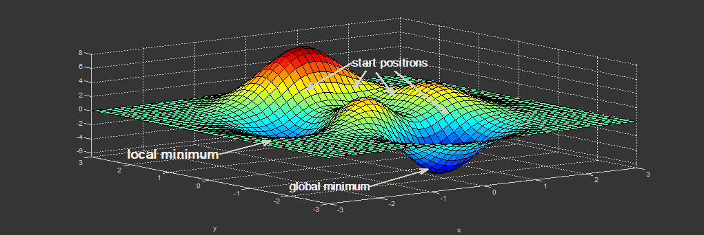
In mathematical optimization there are functions on which new methods are tested.
One such function is the Rosenbrock Function . In the case of a function of two variables, it is defined as

$f (x, y) = (ax) ^ 2 + b (yx ^ 2) ^ 2$

I accepted $a = 0.5, \ b = 0.5$ . Those. function has the form:

$f (x, y) = \ frac {1} {2} (1-x) ^ 2 + \ frac {1} {2} (yx ^ 2) ^ 2$

We will consider the behavior of the function on the interval $-2 \ le x, y \ le 2$

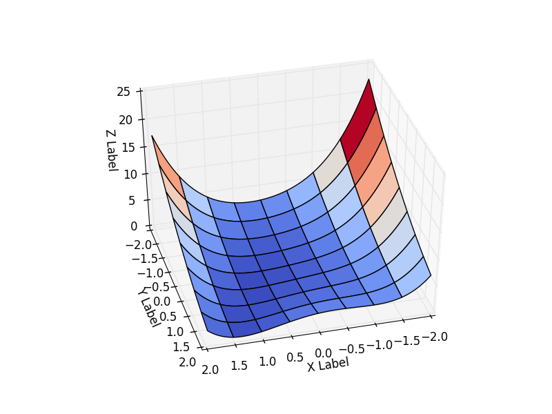
This function is defined non-negatively, has a minimum $z = 0 $ at the point $ (x = 1, y = 1)$
In code, it is easier to encapsulate all the data about the function in one class and take the class of the function that is required. The result depends on the starting point of the optimization. Choose it as $(x = -2, y = -2)$ . As can be seen from the graph, at this point, the function takes the largest value on the interval.

functions.py

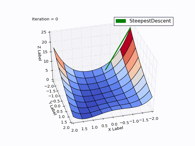
class Rosenbrock: initialPoint = (-2, -2) camera = (41, 75) interval = [(-2, 2), (-2, 2)] """   """ @staticmethod def function(x): return 0.5*(1-x[0])**2 + 0.5*(x[1]-x[0]**2)**2 """    -  - r """ @staticmethod def function_array(x): return np.array([1 - x[0] , x[1] - x[0] ** 2]).reshape((2,1)) @staticmethod def gradient(x): return np.array([-(1-x[0]) - (x[1]-x[0]**2)*2*x[0], (x[1] - x[0]**2)]) @staticmethod def hesse(x): return np.array(((1 -2*x[1] + 6*x[0]**2, -2*x[0]), (-2 * x[0], 1))) @staticmethod def jacobi(x): return np.array([ [-1, 0], [-2*x[0], 1]]) """     : http://www.mathworks.com/help/matlab/matlab_prog/vectorization.html """ @staticmethod def getZMeshGrid(X, Y): return 0.5*(1-X)**2 + 0.5*(Y - X**2)**2

The fastest descent method (Steepest Descent)

The method itself is extremely simple. Accept $F (x) = f (x)$ i.e. objective function coincides with the given one.
Need to find $d_ {ns} (x)$ - direction of the fastest descent of the function $f$ at the point $x$ .
$f (x)$ can be linearly approximated at $x$ :

$f (x + d) \ approx f (x) + \ nabla f (x) ^ Td, \ d \ in R ^ n, || d || \ to 0 \ tag {2}$

$\ lim_ {d \ to 0} f (x) -f (x + d) = - \ nabla f (x) ^ Td \ stackrel {(3.a)} = - || \ nabla f (x) ^ T || \ || d || cos \ theta, \ tag {3}$

Where $\ theta$ - angle between vector $d \ and \ nabla f (x) ^ T$ . $(3.a)$ follows from the dot product

So how do we minimize $f (x)$ then the bigger the difference $(3)$ , all the better. With $\ theta = \ pi$ the expression will be maximally ( $cos \ theta = -1$ , the vector norm is always non-negative), and $\ theta = \ pi$ will only be if vectors $d \ and \ \ nabla f (x) ^ T$ will be opposite, therefore

$d_ {ns} = - \ nabla f (x) ^ T$

We have the right direction, but taking a step long $|| d_ {ns} ||$ You can go the wrong way. Make a step smaller:

$d_ {ns} = - \ alpha \ nabla f (x) ^ T, 0 & lt; \ alpha & lt; one$

In theory, the smaller the pitch, the better. But then the speed of convergence will suffer. Recommended value $\ alpha = 0.05$

In code, it looks like this: first, the base optimizer class. We transfer everything that is needed in the future (Hesse and Jacobi matrices are not needed now, but will be needed for other methods)

 class Optimizer: def __init__(self, function, initialPoint, gradient=None, jacobi=None, hesse=None, interval=None, epsilon=1e-7, function_array=None, metaclass=ABCMeta): self.function_array = function_array self.epsilon = epsilon self.interval = interval self.function = function self.gradient = gradient self.hesse = hesse self.jacobi = jacobi self.name = self.__class__.__name__.replace('Optimizer', '') self.x = initialPoint self.y = self.function(initialPoint) "      " @abstractmethod def next_point(self): pass """     """ def move_next(self, nextX): nextY = self.function(nextX) self.y = nextY self.x = nextX return self.x, self.y

Optimizer code itself:

 class SteepestDescentOptimizer(Optimizer): ... def next_point(self): nextX = self.x - self.learningRate * self.gradient(self.x) return self.move_next(nextX)

Optimization result:

Iteration	X	Y	Z
25	0.383	-0.409	0.334
75	0.693	0.32	0.058
532	0.996	0.990	$10 ^ {- 6}$

It is striking: how quickly the optimization went in 0-25 iterations, in 25-75 it was already slower, and at the end it took 457 iterations to get close to zero. This behavior is very characteristic of the MNS: a very good convergence rate at the beginning, a bad one at the end.

Newton's method

Newton himself searches for the root of the equation, i.e. such $x$ , what $f (x) = 0$ . This is not exactly what we need, because the function may have an extremum not necessarily at zero.

And then there is Newton's Method for optimization . When they talk about MN in the context of optimization, they mean it. I myself, studying at the institute, confused these methods by foolishness and could not understand the phrase "Newton's method has a drawback - the need to count second derivatives."

Consider for $f (x): R \ to R$
Accept $F (x) = f (x)$ i.e. objective function coincides with the given one.

Decompose $f (x)$ in the Taylor series, but unlike the MNS, we need a quadratic approximation:

$f (x + d) \ approx f (x) + f ^ {'} (x) d + \ frac {1} {2} f ^ {' '} (x) d ^ 2, \ d \ in R ^ n, || d || \ to 0 \ tag {4}$

It is easy to show that if $f {'} (x) \ ne 0$ , the function cannot have an extremum in $x$ . Point $x ^ * $ in which $ f {'} (x) = 0$ called stationary .

Differentiate both parts by $d$ . Our goal is to $f (x + d) ^ {'} = 0$ Therefore, we solve the equation:

$0 = f (x + d) ^ {'} = f ^ {'} (x) + f ^ {''} (x) d \\ d_ {n} = - \ frac {f ^ {'} (x )} {f ^ {''} (x)}$

$d_n$ - This is the direction of the extremum, but it can be both a maximum and a minimum. To find out - whether the point $x + d_n$ minimum - you need to analyze the second derivative. If a $f ^ {''} (x) & gt; 0 $, then $ f (x + d_n)$ is a local minimum if $f ^ {''} (x) & lt; 0$ - maximum.

In the multidimensional case, the first derivative is replaced by the gradient, the second - by the Hessian matrix. It is impossible to divide matrices, instead multiply by the opposite (observing the side, since commutativity is absent):

$f (x): R ^ n \ to R \\ H (x) d_ {n} = - \ nabla f (x) \\ d_ {n} = - H ^ {- 1} (x) \ nabla f ( x)$

Similar to the one-dimensional case - you need to check whether we go right? If the Hessian matrix is positively defined , then the direction is correct, otherwise we use the MNF.

In the code:

 def is_pos_def(x): return np.all(np.linalg.eigvals(x) > 0) class NewtonOptimizer(Optimizer): def next_point(self): hesse = self.hesse(self.x) # if Hessian matrix if positive - Ok, otherwise we are going in wrong direction, changing to gradient descent if is_pos_def(hesse): hesseInverse = np.linalg.inv(hesse) nextX = self.x - self.learningRate * np.dot(hesseInverse, self.gradient(self.x)) else: nextX = self.x - self.learningRate * self.gradient(self.x) return self.move_next(nextX)

Result:

Iteration	X	Y	Z
25	-1.49	0.63	4.36
75	0.31	-0.04	0.244
179	0.995	-0.991	$10 ^ {- 6}$

Compare with the MHC. There was a very strong descent to iteration 25 (almost fell from the mountain), but then the convergence slowed down a lot. In MN, on the contrary, we first slowly descend from the mountain, but then we move faster. The MHC took from 25 to 532 iterations to reach zero from $z = 0.334$ . MN optimized $4.36$ for the last 154 iterations.

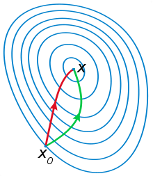
This is a frequent behavior: MN has a quadratic rate of convergence, if you start from a point close to the local extremum. The MNF works well far from the extremum.

The MN uses the curvature information, as was seen in the figure above (smooth descent from the slide).
Another example demonstrating this idea: in the figure below, the red vector is the direction of the MNF, and the green vector is the MN.

[Nonlinear vs linear] least squares method

In MNC we have a model $y = f (\ beta_1, .. \ beta_n; x)$ having $n$ parameters that are configured to minimize

$\ frac {1} {2} \ sum \ limits_ {i = 1} ^ {N} (y_i'-y_i) ^ 2 = \ frac {1} {2} \ sum \ limits_ {i = 1} ^ {N } r_i ^ 2$

where $y_i '$ - $i$ -th observation.

In a linear MNC , we have $ m $ equations, each of which we can represent as a linear equation

$x_i \ beta_1 + x_i \ beta_2 + .. x_i \ beta_n = y_i$

For a linear MNC, the solution is unique. There are powerful methods, such as QR decomposition , SVD decomposition , capable of finding a solution for linear least-squares method for 1 approximate solution of the matrix equation $Ax = b$ .

In nonlinear OLS parameter $\ beta_i$ may itself be represented by a function, for example $\ beta_i ^ 2$ . Also, there may be a product of parameters, for example

$\ beta_1 \ beta_2$

etc.
Here we have to find a solution iteratively, and the solution depends on the choice of the starting point.

The methods below deal with the nonlinear case. But, first, consider the non-isolated MNC in the context of our task - minimizing the function

$f: R ^ 2 \ to R \\ F (x_1, x_2) = f (x_1, x_2) = \ frac {1} {2} (1-x_1) ^ 2 + \ frac {1} {2} (x_2 -x_1 ^ 2) ^ 2 = \ frac {1} {2} r_1 ^ 2 (x_1, x_2) + \ frac {1} {2} r_2 ^ 2 (x_1, x_2)$

Nothing like? This is the form of the MNC! We introduce a vector function $r$

$r: R ^ 2 \ to R ^ 2 \\ r = \ left [\ begin {matrix} 1-x_1 \\ x_2-x_1 ^ 2 \ end {matrix} \ right]$

and we will pick up $x_1, x_2$ so as to solve the system of equations (at least approximately):

$\ begin {cases} r_1 = 1-x_1 = 0 \\ r_2 = x_2 - x_1 ^ 2 = 0 \ end {cases} \\$

Then we need a measure - how good our approximation is. Here she is:

$F (x) = \ frac {1} {2} \ sum_i ^ m r_i ^ 2 (x) = \ frac {1} {2} r ^ T r = \ frac {1} {2} || r || ^ 2 \ tag {5}$

I applied the inverse operation: adjusted the vector function $r$ under the target $F$ . But it is possible and vice versa: if a vector function is given $r: R ^ n \ to R ^ m$ build $F (x)$ from (5). For example:

$r = \ left [\ begin {matrix} x_1 ^ 2 \\ x_2 ^ 2 \ end {matrix} \ right], F (x) = \ frac {1} {2} x_1 ^ 2 + \ frac {1} { 2} x_2 ^ 2$

Finally, one very important moment. The condition must be met $m \ ge n$ otherwise you cannot use the method. In our case, the condition is satisfied

Gauss-Newton Method

The method is based on the same linear approximation, only now we are dealing with two functions:

$r (x + d) \ approx l (d) \ equiv r (x) + J (x) d \\ F (x + d) \ approx L (d) \ equiv \ frac {1} {2} l ^ T (d) l (d)$

Then we do the same as in Newton's method - we solve the equation (only for $L (d)$ ):

$L ^ {''} d_ {n} = -L ^ {'}$

It is easy to show that near $\ text (\ d \ to 0)$ :

$L ^ {''} (d) = J_r ^ T J_r, \ L ^ {'} (d) = J_r ^ T (d) r (d) \\ (J ^ TJ) d_ {n} = -J ^ Tr \\ d_ {n} = - (J ^ TJ) ^ {- 1} J ^ Tr$

Optimizer code:

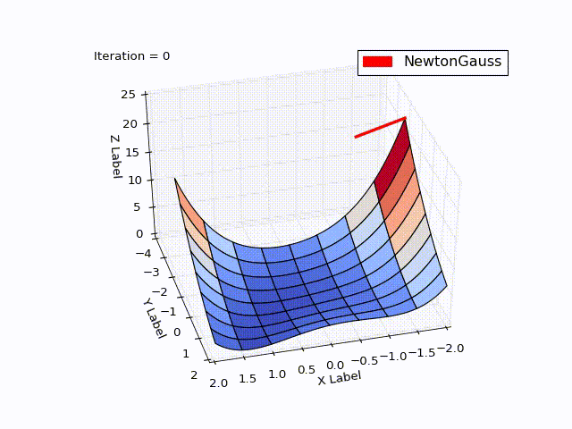
 class NewtonGaussOptimizer(Optimizer): def next_point(self): # Solve (J_t * J)d_ng = -J*f jacobi = self.jacobi(self.x) jacobisLeft = np.dot(jacobi.T, jacobi) jacobiLeftInverse = np.linalg.inv(jacobisLeft) jjj = np.dot(jacobiLeftInverse, jacobi.T) # (J_t * J)^-1 * J_t nextX = self.x - self.learningRate * np.dot(jjj, self.function_array(self.x)).reshape((-1)) return self.move_next(nextX)

The result exceeded my expectations. In just 3 iterations, we came to a point $(x = 1, y = 1)$ . To demonstrate the trajectory of the movement, I reduced the learningrate to 0.2

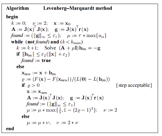
Algorithm of Levenberg - Marquardt

It is based on one of the versions of the Gauss-Newton Method (" damped version "):

$(J ^ T J + \ mu I) d_ {lm} = -J ^ Tr, \ mu \ ge 0$

$\ mu$ called regulation parameter . Sometimes $I$ replace with $diag (J ^ T J)$ to improve convergence.
Diagonal elements $J ^ T J$ will be positive, because element $a_ {ii}$ matrices $J ^ T J$ is the scalar product of a row vector $i$ at $J ^ t$ on myself.

For large $\ mu$ the method of steepest descent is obtained, for small ones the Newton method.
The algorithm itself in the optimization process selects the desired $\ mu$ based on gain ratio , defined as:

$g = \ frac {F (x) - F (x_ {new)}} {L (0) - L (d_ {lm})}$

If a $g & gt; 0$ then $L (d)$ - good approximation for $F (x + d)$ otherwise - you need to increase $\ mu$ .
Initial value $\ mu$ set as $\ tau \ cdot max \ {{a_ {ij}} \}$ where $a_ {ij}$ - matrix elements $J ^ T J$ .
$\ tau$ recommended to appoint for $10 ^ {- 3}$ . The stopping criterion is to reach the global minimum, i.e. $F ^ {'} (x ^ *) = g (x ^ *) = 0$

In optimizers, I did not implement the stopping criterion — the user is responsible for this. I only needed to move to the next point.

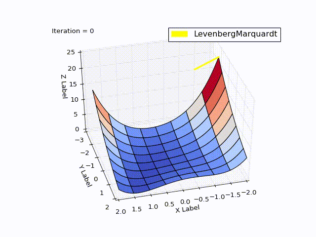
 class LevenbergMarquardtOptimizer(Optimizer): def __init__(self, function, initialPoint, gradient=None, jacobi=None, hessian=None, interval=None, function_array=None, learningRate=1): self.learningRate = learningRate functionNew = lambda x: np.array([function(x)]) super().__init__(functionNew, initialPoint, gradient, jacobi, hessian, interval, function_array=function_array) self.v = 2 self.alpha = 1e-3 self.m = self.alpha * np.max(self.getA(jacobi(initialPoint))) def getA(self, jacobi): return np.dot(jacobi.T, jacobi) def getF(self, d): function = self.function_array(d) return 0.5 * np.dot(function.T, function) def next_point(self): if self.y==0: # finished. Y can't be less than zero return self.x, self.y jacobi = self.jacobi(self.x) A = self.getA(jacobi) g = np.dot(jacobi.T, self.function_array(self.x)).reshape((-1, 1)) leftPartInverse = np.linalg.inv(A + self.m * np.eye(A.shape[0], A.shape[1])) d_lm = - np.dot(leftPartInverse, g) # moving direction x_new = self.x + self.learningRate * d_lm.reshape((-1)) # line search grain_numerator = (self.getF(self.x) - self.getF(x_new)) gain_divisor = 0.5* np.dot(d_lm.T, self.m*d_lm-g) + 1e-10 gain = grain_numerator / gain_divisor if gain > 0: # it's a good function approximation. self.move_next(x_new) # ok, step acceptable self.m = self.m * max(1 / 3, 1 - (2 * gain - 1) ** 3) self.v = 2 else: self.m *= self.v self.v *= 2 return self.x, self.y

The result was good too:

Iteration	X	Y	Z
0	-2	-2	22.5
four	0.999	0.998	$10 ^ {- 7}$
eleven	one	one	0

When learningrate = 0.2:

Method comparison

Method name	Objective function	Virtues	disadvantages	Convergence
The fastest descent method	differentiable	- wide range of applications -simple implementation - low price per iteration	- the global minimum is searched worse than in other methods -low convergence rate near extremum	local
Newton's method	twice differentiable	-high rate of convergence near the extremum - uses curvature information	-function must be twice differentiable will return an error if the Hesse matrix is degenerate (does not have an inverse) -There is a chance to go wrong if far away from the extremum.	local
Gauss-Newton Method	nonlinear OLS	- very high convergence rate -Works well with the task of curve-fitting	- columns of matrix J should be linearly independent - imposes restrictions on the type of the objective function	local
Algorithm of Levenberg - Marquardt	nonlinear OLS	-labability among the considered methods -The greatest chance of finding a global extremum - very high convergence rate (adaptive) -Works well with the task of curve-fitting	- columns of matrix J should be linearly independent - imposes restrictions on the type of the objective function -complicated implementation	local

Despite the good results in the concrete example, the considered methods do not guarantee global convergence (to find which is an extremely difficult task). An example of the few methods that can still achieve this is the basin-hopping algorithm.

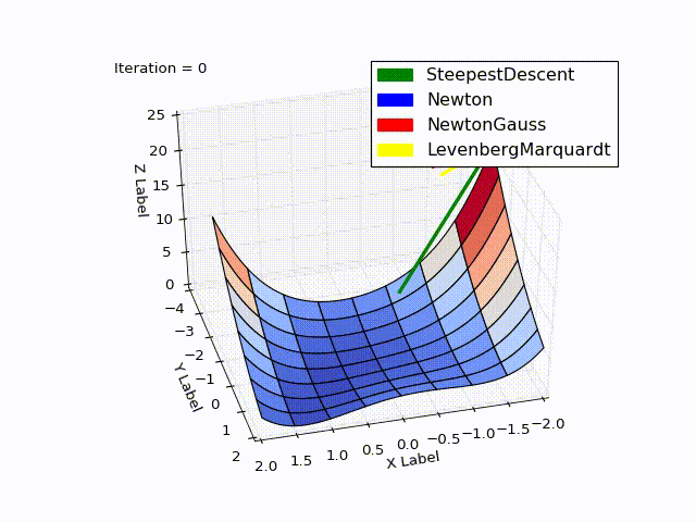
Combined result (specially reduced speed of the last two methods):

Sources can be downloaded from github

Sources

K. Madsen, HB Nielsen, O. Tingleff (2004): Methods for non-linear least square
Florent Brunet (2011): Basics on Continuous Optimization
Least Squares Problems

Source: https://habr.com/ru/post/308626/

All Articles

The Levenberg-Marquardt algorithm for the nonlinear least squares method and its implementation in Python

More articles: