Mathematics for artificial neural networks for beginners, part 3 - gradient descent continued

Part 2 - Gradient Descent Start

In the previous part, I began to analyze the optimization algorithm called gradient descent. The previous article broke down on writing a variant of the algorithm called packet gradient descent.

There is another version of the algorithm - stochastic gradient descent. Stochastic = random.

,

{
for i in train_set
{

}
}

Also recall what the batch looks like:
')
,
{

}

The formulas are similar, but, as you can see, the packet gradient descent calculates one step, using the entire data set at once, whereas the stochastic step uses only 1 element per step. You can cross these two options by getting a mini-batch descent, which processes, for example, 100 elements at once, but not all or one.

These two options behave similarly, but not equally. The batch descent really follows the direction of the fastest descent, whereas the stochastic descent, using only one element from the training sample, cannot correctly compute the gradient for the entire sample. This distinction is easier to explain graphically. To do this, I modify the code from the first part, in which the linear regression coefficients were calculated. The cost function for it is as follows:

As you can see, this is a slightly elongated paraboloid. And also his “top view”, where the true minimum, found analytically, is marked with a cross.

First, let's look at how the package descent behaves:



Due to the fact that the paraboloid is elongated, a “ravine” passes through its “bottom”, into which we fall. Because of this, the last steps along this ravine are very small, but nevertheless, sooner or later the gradient descent will reach a minimum. The descent takes place along the anti-gradient line, each step approaching the minimum.

Now the same function, but for stochastic descent:


The definition says that only one element is selected — in this code, each subsequent element is selected at random.


As can be seen, in the case of the stochastic variant, the descent does not go along the line of the antigradient, but in general it is not clear how - every step deviates in a random direction. It may seem that such random jerky movements to the minimum can only come by chance, but it was proved that the stochastic gradient descent converges almost certainly. A couple of links , for example .


On 200 elements, there is almost no difference in speed, however, by increasing the number of elements to 2000 (which is also very small) and adjusting the learning speed, the stochastic version beats the batch as it wants. However, due to the stochastic nature, sometimes the method misses, oscillating near the minimum without the possibility to stop. Something like this:



This fact makes pure implementation inapplicable. To somehow call to order and reduce the "chance" you can reduce the speed of learning. In practice, mini-batch variation is used - it differs from the stochastic one in that instead of one randomly selected element, more than one is chosen.

Quite a lot has been written about the difference, pros and cons of these two approaches, to summarize in brief:

- Batch descent is good for strictly convex functions, because it is confidently striving for a minimum of global or local.
- Stochastic, in turn, works better on functions with a large number of local minima - every step is a chance that the next value will “knock” out of the local pit and the final solution will be more optimal than for the package descent.
- Stochastic is calculated faster - not all elements from the sample are needed at every step. The entire sample may not get into the memory. But more steps are required.
- For stochastic, it is easy to add new elements while working (“online” training).
- In the case of mini-batch, you can also vectorize the code, which will significantly speed up its execution.

Also, there are many modifications of gradient descent - momentum, steepest descent, averaging, Adagrad, AdaDelta, RMSProp and others. Here you can see a brief overview of some. Often they use the gradient values ​​from the previous steps or automatically calculate the best speed value for a given step. Using these methods for a simple smooth OLS function does not make much sense, but in the case of neural networks and networks with a large number of layers \ neurons, the cost function becomes quite sad and the gradient descent can get stuck in a local well without reaching an optimal solution. For such problems are suitable methods on steroids. Here is an example of a simple function to minimize (two-dimensional linear regression with OLS):

And an example of a non-linear function:



Gradient descent is a first order optimization method (first derivative). There are also many second-order methods — for them it is necessary to calculate the second derivative and build the Hessian (a rather expensive operation - ). For example, the gradient descent of the second order (the learning rate was replaced by the Hessian), BFGS, conjugate gradients, the Newton method and a huge number of other methods . In general, optimization is a separate and very wide layer of problems. However, here is an example (though only a presentation) of the work + video of Jan Lekun , in which he says that you can not soar and just use gradient methods. Even considering that the 2007 presentation, many recent experiments with large ANNs used gradient methods. For example .

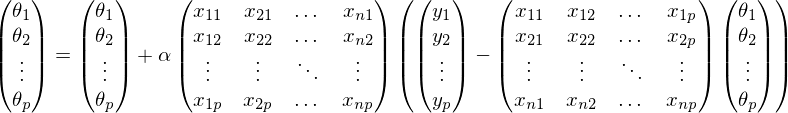
You won't get far on bare cycles - the code needs to be vectorized. The main algorithm for vectorization is packet gradient descent, with the proviso that where k is the number of elements in the test set. Thus, vectorization is suitable for the mini-batch method. Like last time, I'll write out everything in the vectors that have been opened. Note that the first matrix is ​​transposed -



For proof, let's go a couple of steps in the opposite direction:





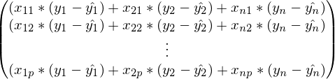
In the previous formula, in each line the index j is fixed, and i - varies from 1 to n. Curtailed amount:



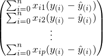
This expression is exactly the same as in the definition of gradient descent. Finally, the final step is the folding of vectors and matrices:



The cost of one such step - where n is the number of elements, p is the number of signs. Much better . An expression identical to this also occurs:



Notice that the predicted value and the real value were reversed, which led to a change in sign before the learning speed.

"To run the examples you need: numpy, matplotlib.
»Materials used in the article - github.com/m9psy/neural_network_habr_guide