R and Spark

Spark , an Apache project designed for cluster computing, is a fast and versatile data processing environment, including machine learning. Spark also has an API for R ( SparkR package), which is included in the Spark distribution itself. But, in addition to working with this API , there are two more alternative ways to work with Spark in R. So we have three different ways to interact with the Spark cluster. This post provides an overview of the main features of each of the methods, and using one of the options, we will build the simplest model of machine learning on a small amount of text files (3.5 GB, 14 million lines) on the Spark cluster deployed in Azure HDInsight .

Spark Interaction Overview

In addition to the official SparkR package, the capabilities in machine learning of which are weak (in version 1.6.2 there is only one model, in version 2.0.0 there are four of them), there are two more options for access to Spark .

The first option is to use a product from Microsoft - Microsoft R Server for Hadoop , which has recently integrated support for Spark . Using this product, you can perform calculations for the same R functions, in the context of local calculations, Hadoop ( map-reduce ) or Spark . In addition to the local installation of R and access to the Spark cluster, the Microsoft Azure HDInsight cloud service allows you to deploy ready-made clusters, and, in addition to the usual Spark cluster, you can also deploy the R Server on Spark cluster. This service is a Spark cluster with a pre-installed R server for Hadoop on an additional, border node that allows you to immediately perform calculations, both locally on this server, and switch to the Spark or Hadoop context. The use of this product is quite well described in the official documentation for HDInsight on the Microsoft website.

The second option is to use the new sparklyr package, which is still under development. This product is developed under the auspices of RStudio - the company, under the wing of which some of the most useful and necessary packages are released - knitr, ggplot2, tidyr, lubridate, dplyr and others, so this package can become another leader. So far this package is poorly documented, since it has not yet been officially released.
')
Based on the documentation and experiments with each of these methods of working with Spark , I prepared the following table (Table 1) with generalized functionality of each of the methods (also added SparkR 2.0.0 , in which there were a few more features).


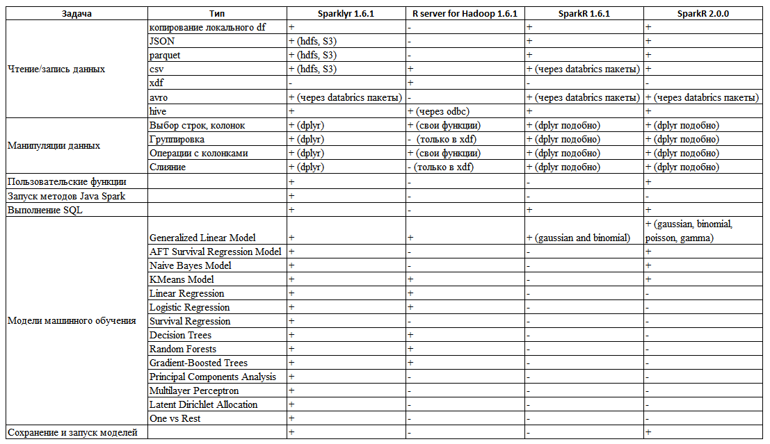
Table 1. Overview of the possibilities of different ways to interact with Spark

As can be seen from the table, there are no tools that fully realize the necessary needs out of the box, but the sparklyr package compares favorably with SparkR and R Server . Its main advantages are reading csv , json , parquet files from hdfs . Fully dplyr- compatible data manipulation syntax — including filtering, column selection, aggregation functions, data merging capabilities, column name modification, and more. Unlike SparkR or R server for Hadoop , where some of these tasks are either not performed or are very inconvenient (in R server for Hadoop, data merging for objects does not exist at all, it is supported only for the xdf embedded data type). Another advantage of the package is the ability to write functions for running Java methods directly from R code.

Example

count_lines <- function(sc, file) { spark_context(sc) %>% invoke("textFile", file, 1L) %>% invoke("count") } count_lines(sc, "/text.csv") 

Because of this, you can implement the missing functionality of the package using the existing java methods in Spark or by implementing them yourself.

And, of course, the number of machine learning models is much larger than that of SparkR (even in version 2.0) and R server for Hadoop . Therefore, we will opt for this package as the most promising and convenient to use. The Spark cluster was deployed using the Azure HDInsight cloud service offering deployment of 5 cluster types ( HBase , Storm , Hadoop , Spark , R Server on Spark ), in different configurations with minimal effort.

Resources used

• HDInsight Apache Spark 1.6 cluster on Linux (cluster deployment is described in detail in the Microsoft Azure documentation)
• R 3.3.2 installed on the head node
• RStudio preview edition (additional features for sparklyr), also installed on the head node
• Putty client to establish a session with the cluster head node and tunnel the RStudio port to the local host port (setting up RStudio and its tunneling is described in the Microsoft Azure documentation)

Environment setup

First we deploy the Spark cluster - I chose a configuration with 2 head nodes D12v2 and 4 work nodes D12v2. (D12v2: 4 cores / 28 GB of RAM, 200 GB disk, this configuration is not entirely optimal, but it is suitable for demonstration of the syntax sparklyr ). Description of the deployment of different types of cluster and work with them is described in the documentation on HDInsight . After successfully deploying the cluster, using an SSH connection to the working node, install R and RStudio there, with the necessary dependencies. RStudio it is advisable to use the preview editions, since it has additional features for the sparklyr package - an additional window that displays the original data frames in Spark, and the ability to view their properties or themselves. After installing R, R Studio, we re-establish the connection using tunneling to localhost: 8787 .

So, now in the browser at localhost: 8787 we connect to RStudio and continue to work.

Data preparation

All the code for this task is given at the end of this post.

For this test task, we will use the NYC Taxi dataset csv files located at NYC Taxi Trips . The data is information about taxi rides and their payment. For familiarization purposes, we limit ourselves to one month. Building a model on the same complete dataset, but using R Server for Hadoop (in the context of Hadoop ), is described in the following article: Exploring NYC Taxi Data with Microsoft R Server and HDInsight . But there the reading of files, all the preprocessing - filtering the data, merging the tables was done in Hive , and in the R Server they only built the model, here everything is done on a regular R using sparklyr .

Having moved both files to the hdfs of the Spark cluster, and using the sparklyr function, we read these files.

Data manipulation

Files for trips and tariffs are linked by key - the columns " medallion ", " hack_licence " and " pickup_datetime ", so we will perform the attachment on the left to the data frame, data frame fare . After combining data and manipulations, we save the data frame in parquet format. Before building a model, we will look at the data, for this we will create a sample of 2000 random observations and pass them to R using collect. On this small sample, a standard ggplot2 diagram was constructed (the tip depends on the fare, indicating the size of the point — the distance of the route and the color of the point by the number of passengers, and divided into a grid by type of payment and taxi operator) (Fig. 1).


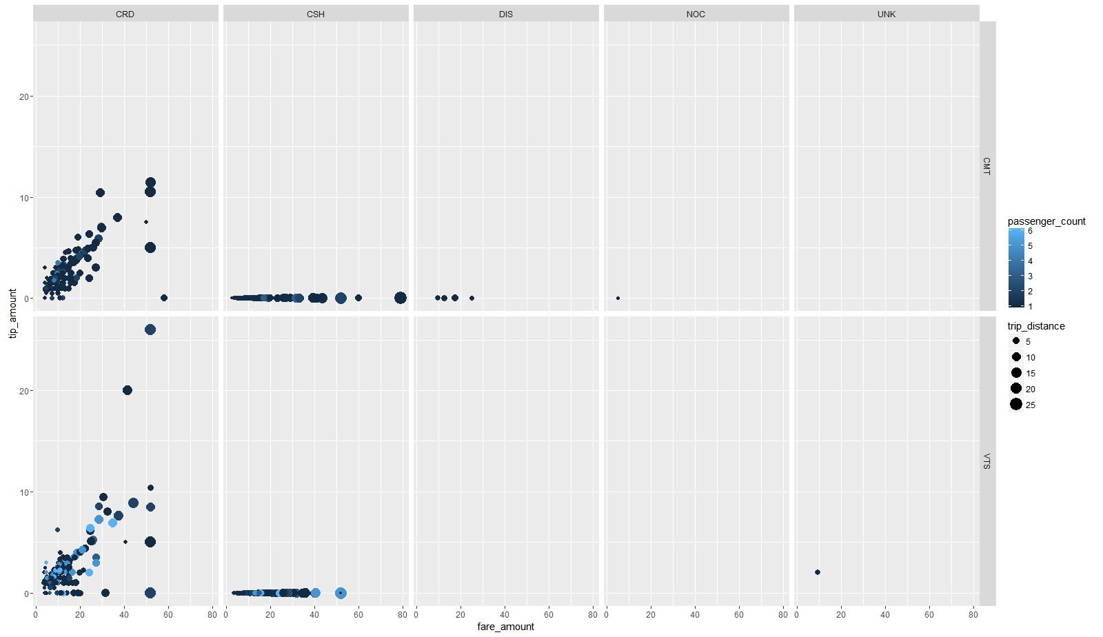
Figure 1 Chart showing the main dependencies

It shows that there is a dependence (linear, as “standard”% of the bill) of the tip size on the fare, most of the payments are made using a credit card (CRD panel) and cash (CSH panel), and that when paying cash in tips They are absent (this is probably due to the fact that when paying in cash, tips are already included in the cost of payment, and when paying with a card there is no). Therefore, in the sample for training we leave only those trips that were paid by credit card. Using the convenient dplyr syntax and magrittr Piping , we merge the combined dataframe further along the chain: subsequent selection of rows (excluding outliers and illogical values) and columns (leaving only those necessary for building the model), passing the final dataset to the linear regression function. To train the model, we use 70% of all data, for the test the remaining 30%. For this problem we use simple linear regression. The dependency we want to detect is the size of the tip on the parameters of the trip. The model on these data is quite degenerate and not quite correct (there are a large number of tips equal to 0), but it is simple, it will show the interpretable coefficients of the model and will allow you to demonstrate the basic features of sparklyr . We will use the following predictors in the model: vendor_id is the identifier of the taxi operator, passenger_count is the number of passengers, trip_time_in_secs is the trip time, trip_distance is the trip distance, payment_type is the type of payment, fare_amount is the price of the trip, surcharg e is the charge. As a result of training, the model has the following form:

 Call: ml_linear_regression(., response = "tip_amount", features = c("vendor_id", "passenger_count", "trip_time_in_secs", "trip_distance", "fare_amount", "surcharge")) Deviance Residuals: (approximate): Min 1Q Median 3Q Max -27.55253 -0.33134 0.09786 0.34497 31.35546 Coefficients: Estimate Std. Error t value Pr(>|t|) (Intercept) 3.2743e-01 1.4119e-03 231.9043 < 2e-16 *** vendor_id_VTS -1.0557e-01 1.1408e-03 -92.5423 < 2e-16 *** passenger_count -1.0542e-03 4.1838e-04 -2.5197 0.01175 * trip_time_in_secs 1.3197e-04 2.0299e-06 65.0140 < 2e-16 *** trip_distance 1.0787e-01 4.7152e-04 228.7767 < 2e-16 *** fare_amount 1.3266e-01 1.9204e-04 690.7842 < 2e-16 *** surcharge 1.4067e-01 1.4705e-03 95.6605 < 2e-16 *** --- Signif. codes: 0 '***' 0.001 '**' 0.01 '*' 0.05 '.' 0.1 ' ' 1 R-Squared: 0.6456 Root Mean Squared Error: 1.249 

Using this model, we predict the values ​​on the test sample.

findings

This article presents the main functionalities of the three ways of interacting with Spark in R and provides an example that implements reading files, their preprocessing, manipulating them and building a simple machine learning model using the sparklyr package.