Navigator 2GIS: Extrapolation of the position of the car

In the application 2GIS now have a navigator. We learned to “go” on the track, voice maneuvers, automatically rebuild the route, calculate the time on the way, bring the user to the entrance to the building or organization, taking into account fences and barriers - all in an honest offline. Traffic jams (except that they need the Internet), bridges and streets that have been blocked have been considered for a long time. While in our navigator - the necessary minimum. A little later we will teach him to warn about too high speed, speed bumps and traffic police cameras, set up the night mode, make the routes on toll and dirt roads optional. To use it, you need to update 2GIS in your smartphone or download it in the AppStore or Windows Store . For Android, the update comes out gradually, starting from August 22 (will be available to the entire audience by September).

And today we will tell how the 2GIS navigator predicts the position of the car and smoothly moves the arrow along the route. After all, the quality of the user's route guidance determines the ergonomics of the interface of any modern navigator, the simplicity of orientation on the terrain and the timeliness of maneuvers.

Most of the time, the driver of the car has to follow the road, so even a quick glance at the screen of the device with the navigator program should be enough to get the most accurate and timely information about its location relative to the route and surrounding objects. This seemingly simple functionality requires solving a number of technical problems for its implementation. Some of them we consider.
')

GPS marker and route

To mark the user's location on the map, many navigators (and ours are no exception) use a special GPS marker in the form of an arrowhead or simply a triangle, which intuitively indicates the direction of motion. In addition, the marker should be clearly visible on the map, so its color is usually very different from the background, edges are additionally circled, etc.

In the simplest case, you can display the position of the device on the ground, reading the coordinates from the GPS sensor and placing the marker in the appropriate place on the map. Already here we are confronted with the first problem - the measurement error, which even in conditions of a good signal may well reach 20–30 meters.

To answer the usual question “Where am I?” This way of displaying will be quite sufficient, especially if around the marker we also draw a circle of accuracy with a radius equal to the estimated error. However, to navigate, you need to come up with something better, because a driver moving along a city street is unlikely to be satisfied with a GPS marker located inside a neighboring house or, even worse, on some intra-block passage.

The route built by the program to the destination point and always present in the navigation script helps to solve the problem. With the help of some tweaks, we can “pull” a point on the map to the route, leveling some of the measuring error of the GPS sensor. In the first approximation, a draw can be viewed as projecting a point onto a route line. Consideration of the same nuances, as well as ways to detect a route detour, unfortunately, is beyond the scope of this article.

By adopting the indicated draw technique, we can abstract away from the two-dimensional geographic coordinates (latitude-longitude or any other) and move on to a one-dimensional coordinate — an offset from the beginning of the route, measured, for example, in meters. Such a transition simplifies both theoretical models and calculations performed on user devices.

Display geo-location in time

The discrete nature of the receipt of data from the GPS sensor is another problem when implementing user guidance along a route. In the ideal case, the coordinates are updated once per second. Consider several options for displaying the geo-location in time and choose the most suitable for our tasks.

1. The easiest way is to receive each new sample from the sensor, immediately draw to the route and display the corresponding location on the map. Among the advantages, it is worth noting the exceptional ease of implementation, high accuracy in a certain sense (after all, here we simply display satellite data without making any serious changes to them) and minimal computational complexity. The main drawback is that the marker in this case does not move around the map in the usual sense, but “teleports” from point to point. In the main navigation scenarios, the camera (virtual observer - a term from the field of computer graphics) is tied to the GPS marker, so its teleportation like this leads to a sharp “misalignment” of the map along the route and, as a result, to the driver’s disorientation, especially at high speeds, when Between the geo-location counts, the car travels a considerable distance. Our task is to help the user, and not confuse him, so this flaw is already enough to exclude this option from consideration.

The only way to avoid disorientation is to move the GPS marker smoothly, without “teleportation”, which means that you need to move it much more often than geo-location counts come. To ensure such a movement, it is necessary to somehow calculate the intermediate points between the actual readings from the sensor and use them until the next reading is obtained. The specific approach to the calculation of these intermediate points should be given special attention, since it ultimately greatly affects the overall ergonomics of the navigator program.

2. The second way to display the user's location is associated with the most obvious approach to the generation of intermediate points - interpolation between the last real GPS samples. The point is to move the marker from the penultimate count to the last for some specified time, calculating intermediate points with the required frequency from one of the known mathematical functions (the simplest option is linear interpolation ). Using the navigator with this method is much more convenient, but it also has disadvantages.

One of the most innocuous is the need to pre-set the interpolation time. Installing it in one second will work well only in the ideal case mentioned above, when exactly so much time will pass between the GPS samples. If less time passes — it doesn't matter, you can simply start moving from your current position to a new target. But if more - the marker will have to stand still and wait for new coordinates from the sensor, although the user's car may well move at this time.

There is a more serious problem. At the moment of arrival of a new reference, the marker is at best located at the previous real point. From the user's point of view, we introduce another positioning error, the value of which is not less than the distance traveled by the vehicle during the time between readings. At a speed of 100 km / h, this value reaches almost 28 meters, which, coupled with the possible measurement error, makes the information provided to the user unreliable, to say the least.

We could make a huge GPS marker and block a quarter of the screen with it, carefully masking the flaws of the described positioning method, but going to a direct forgery would be a disrespect to users and to ourselves. Accuracy and timeliness of the displayed data is no less important criterion when developing a navigator than external beauty and smooth movement.

3. Taking into account the positioning accuracy requirement that has appeared, it is worth noting that now we are required to locate the marker at a point as close as possible to this new countdown, shortly before the arrival of the new GPS readout. That is, in fact, look into the future, albeit briefly. Although humankind has a bad time with the invention of the time machine, things are still there for us. The movement of the car is inert, so the speed and direction of its movement cannot change instantly, and if so, we can try with some accuracy to predict where the user will be in the interval between the last countdown of the position and the future. If we manage to ensure that the prediction error in most cases will be less than the error of the second method, then we will greatly facilitate the life of the users of our navigator.

This kind of prediction in the exact sciences is called extrapolation. It is this way that we will go in an attempt to develop a third method of route guidance that satisfies all the criteria listed above. Next, we will have to resort to a more formal language of presentation, as soon as we speak about mathematical models.

Route guidance with position extrapolation

It was mentioned earlier that due to the user’s geo-location draw to the navigation route, we can move from two-dimensional geographic coordinates to a one-dimensional coordinate - offset relative to the beginning of the route (for brevity, we will use the term “offset” without further specification).

Let us recall the data arriving to us and enter notations for them:

- real offset readings obtained by the draw of the GPS position to the route line;
- the arrival time of the corresponding offset samples.
This, in fact, the list of input data ends. We'll have to squeeze the maximum useful information out of them.

Ultimately, we need to build an offset extrapolation function , which will be close to the real dynamics of the car and at the same time ensure the smoothness of the GPS marker movement throughout our route (its length will not affect anything, since the completion of the route is processed separately, therefore we will conditionally consider the route to be infinite). Smoothness is enough to ensure good visual smoothness. , that is, neither the position nor the speed of the marker should change abruptly. In other words, the function must be continuous with its first derivative (hereinafter - in time) throughout the domain of definition.

Note that each real offset reading carries substantially new motion information. For example, if for a long time the car drove evenly and then began to accelerate, the navigator can “feel” the acceleration only with the arrival of the next countdown. Since we cannot look into the future for an arbitrarily long period of time, all incoming new GPS readings will generally change the behavior of the desired function. That does not allow to set it with a single analytical expression. Instead, try to define the function piecewise. To do this, we solve the simpler problem first.

Immediate piecewise extrapolation

We construct such an extrapolation displacement function so that after countdown, its values ​​predicted the actual location of the user for a sufficient time before the arrival th countdown. All useful data we possess is a sequence of readings to together with the time of receipt of each of them.

Remembering the finite differences, we note that we have the opportunity to estimate the speed of the vehicle in moment of time, dividing the length of the segment between the last and the penultimate offset by the corresponding time interval:


where - an estimate of the speed of the readings, and - derivative of extrapolation function that we are trying to build.

Similarly for higher order derivatives - acceleration, jerk, etc .:


As can be seen from these formulas, to obtain an estimate of higher and higher derivatives of the displacement, it is necessary to take into account more and more samples preceding the current one: to determine the speed two counts are needed, three are needed for acceleration, four are needed for a jerk, etc. On the one hand, the more dynamic characteristics of the movement we take into account in our forecast, the greater the modeling capacity we will get; on the other hand, the useful information contained in more and more “old” readings dramatically loses its relevance. For example, the fact that we were traveling at a speed of 30 km / h a minute ago would not help us at the current time: since then, it was possible to accelerate several times, slow down or stop altogether. For this reason, the estimates of higher and higher displacement derivatives are getting farther from reality; In addition, the contribution of the error in calculating a certain derivative to the general analytical model of bias also increases with an increase in the order of this derivative. If this is the case, then, starting with a certain order, the dynamic characteristics, estimated using finite differences, instead of specifying, will only spoil our model.

According to the results of checks on real data, it turned out that the assessment of a jerk , especially in cases of the “average” quality of the GPS signal, is already bad enough for it to do more harm than good. On the other hand, fortunately, the most frequent scenarios of car dynamics are rest, uniform and uniform motion, described by polynomial equations of the 0th, 1st, and 2nd degrees of time, respectively.

It turns out that a quadratic model of uniformly alternating traffic will be quite enough for us to describe most of the road situations, and for it we just have more or less qualitative assessments of the dynamic characteristics - speed and acceleration. Recalling the school course of physics, we can already in outline form an analytical expression for the desired extrapolation function:


It remains to do just one step: the scope starts from the moment of time therefore, it is more convenient to calculate time in calculations from the same moment.

As a result, the function will take the form:


A remarkable feature of this function is its smoothness over the entire domain, which, as mentioned earlier, is included in the formulation of our problem.

Now, take some real offsets from the device and try to extrapolate them at each interval (although defined to at the moment of arrival We will immediately move on to the next function. because it has more recent data):



Let's make a reservation that for clarity, the data was taken with a relatively low quality of the GPS signal, however, the situation in the figure is very real and can arise for any user.

The smoothness of each extrapolation polynomial perfectly visible at the corresponding time interval, but the trouble is that at the junctions of the intervals the common gray curve suffers gaps, sometimes quite noticeable.

Let's call the gap in moment of time by extrapolation error . Indeed, it is this value that shows how inaccuracy each of our forecasts has towards the end of its time interval. You can calculate the error value using the following expression:


Alas, reduce the error to zero by varying the functions themselves. , we can not, because it would be equivalent to one hundred percent accuracy of vision of the future. So, to solve our original problem of constructing a single function you have to somehow “glue” the piecewise extrapolation polynomials between each other, that is, correct the errors that occur at the joints.

Error Correction Approach

In accordance with the notation chosen above, one can informally say that by the time a new reference comes we are at a point i.e. shifted relative to the real position by the amount of error accumulated by the time previous extrapolation polynomial .

On the one hand, from the point of view of compliance with the data provided to the user of reality, the best way to correct the error there will be a function gap to the starting point of the next polynomial however, we cannot do this, because in this case we will again “teleport” the marker on the map and disorient the driver.

Obviously, if the instantaneous change in value Invalid, error correction will take some non-zero time. It is also clear that it is desirable to complete the correction of the error before the next reading comes in order to prevent the accumulation of error.

Due to the stochastic nature of the time intervals between offsets, it is not possible to reliably determine the exact time of the correction. Therefore, in the first approximation, we fix the error correction time in the form of a certain constant value, the specific value of which we will select in the future by practical consideration.

If you speak informally again, to correct the error is required from the point during smoothly “return” to the next extrapolation polynomial - curve .

To describe the error correction process, it is convenient to introduce separate correction functions. so that at time the corresponding correction function has a value , and from the moment became zero:


If we add such a correction function with the corresponding interpolation polynomial, then at key points and we will provide offset error correction:


Let's call the corrected offset function the sum of the extrapolation polynomial and the corresponding correction function:


Note that due to the properties of the correction functions described above, we obtained a very important property of the functions - they are already “stitched by offset”, i.e. do not tolerate gaps in the points :


The set of adjusted functions could claim to be the desired displacement model , defined at all times, if not for one circumstance: despite the absence of discontinuities at the points , the derivatives of this set of functions are generally still broken.

Specifically, we are interested in breaking the first derivative - the speed, because the initial requirements contain a condition for ubiquitous smoothness i.e. condition of ubiquitous speed continuity. With this in mind, it is necessary to expand the requirements for correction functions. , to "sew" more and derivatives of the corrected functions :


This equation is a condition for the smoothness of the set of corrected functions. Substituting the definition of the adjusted functions in both sides of the equation, we obtain


Earlier we mentioned that after the expiration of the correction time the correction function takes on zero values. Add one more requirement to the correction function - let its derivative after zero of the correction time also take zero values:


Then, assuming that the correction time is always less than the interval between samples, we can assume that the derivative correction function by the time of the next count already go to zero. Then, returning to the condition of smoothness, we get:


Express from here :



notice, that is an estimate of speed, made with the help of finite differences, we substitute it:


The right-hand side is an extrapolation error of speed — the difference between the speed obtained from the previous extrapolation polynomial and the “real” speed reference. Now we can put together the boundary conditions for the correction functions:


Words can describe them like this - it is necessary to find the correction function in order to:

• at the beginning of the correction interval, its value coincided with the bias extrapolation error;
• at the beginning of the correction interval, the value of its derivative coincided with the velocity extrapolation error;
• at the end of the correction interval and further, the value of the function itself and its derivative was zero.

Selection of error correction function

It should be noted that to obtain a single analytical expression for the correction functions , exactly satisfying the above four conditions is very difficult. The problem lies in the part of the domain that goes after the correction time expires. , - it is necessary to achieve zero values ​​of the function and its derivative on the entire remainder of the numerical axis. To simplify the task, we reduce the domain of definition of the desired analytical expression of the correction function to the correction interval. , and after its upper boundary we will consider the value of the function and its derivative to be trivially zero (good, at the level of the program code we have this possibility due to the presence of branching).

Formally, taking this technique into account, the correction function is piecewise — some expression for the correction interval and a constant 0 further, however, subject to the boundary conditions at the point neither the correction function itself nor its first derivative will break. Since the discontinuities of the higher derivatives do not interest us (they do not spoil the smoothness of the desired function ), we will not mention the zero “tail” of the correction function in the future, and reformulate the boundary conditions in a more convenient form:


Denote the error of the extrapolation of speed through :


Now you need to define an analytical expression for .Due to ergonomic program requirements, in addition to the boundary conditions, it is necessary that the correction function has as few extremes and excesses as possible in the correction interval - so that the GPS marker “does not twitch”.

The simplest function suitable for these requirements is again a polynomial - a polynomial of the smallest possible degree of time (theoretically, the sine also has similar characteristics among the elementary functions, but it is more expensive to calculate its value in terms of CPU time).

Since the boundary conditions are a system of four non-trivial equations, the minimum degree of the polynomial that provides sufficient parametrization of the correction function is the third. Considering that when constructing an analytical expression forit is more convenient to count the time from the moment of the ith reference (exactly the same as in the definition , the desired polynomial takes the following form:


Substituting this expression into the system of boundary conditions and solving it with respect to constants and , we get the following values:


As a result, if the correction functions are determined in the manner described, the corrected functions are merged into a single extrapolation function , smooth at all points in time. We will not give the full expression for its cumbersomeness.

Note: the last inaccuracy remained in the assumption when choosing the correction time - our reasoning was built in light of the condition that there will always be less than the interval between readings:


A nice feature of the constructed model is that it is enough for us to choose in such a way that it does not exceed the average time between samples: if the individual intervals are smaller , then the part of the error that we did not have time to correct for too short an interval will be corrected on one of the following. To do this, it will suffice to calculate the extrapolation error not by the usual extrapolation function , but by the corrected :


The figure below shows an example of a graph of the final extrapolation function , built on real data: The



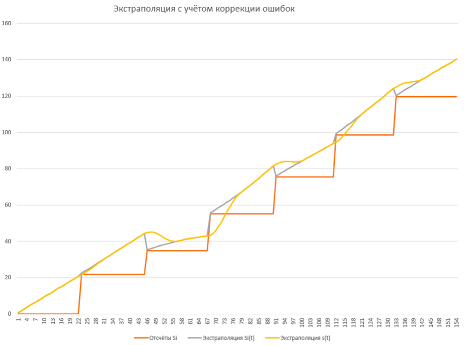
formal problem is solved, the resulting curve satisfies all the specified conditions, and it looks quite nice. It would be possible to relax on this, but the features of the real world present certain difficulties for the constructed idealized system.

Let us consider some of them in more detail, making a reservation that all the decisions made later are implemented directly in the program code outside of the mathematical model.

Adaptation of the mathematical model to real conditions

The prohibition of movement of the marker in the opposite direction

In the last graph, you can see that in some cases, the function starts to decrease, even when the user is driving only forward along the route based on real counts. This happens when our forecast strongly overestimates the speed of movement. On the other hand, in reality, the car moves in the opposite direction only for two reasons: the driver actually turned on the rear gear and went back (a very rare case), or performed a U-turn.

In the case of a turn, the road situation changes significantly, which requires rebuilding the navigation route; This is a separate topic and does not fit into the framework of this article.

If we use the results of position extrapolation bydirectly, then from all movements of the marker in the direction of the beginning of the route, the disappearing minority will correspond to the real movement of the car in the same direction. In light of this, it was decided to ban the marker from moving back without rebuilding the route, so as not to mislead users.

Such a rigid condition is difficult to describe in the language of mathematics, but it is relatively easy to implement in the program code. To begin with, we will take into account the discrete nature of model time — due to the peculiarities of the functioning of computers, we will in any case obtain extrapolation results at some selected points in time.

If this is the case, it will not be difficult to ensure that the extrapolated offset does not decrease: it is enough to compare the new value obtained with the previous one, and if the current value is less, then replace it with the previous one. Despite the apparent rudeness of this technique, we will not break the smoothness of the extrapolation function, because in order to start moving back along the smooth function, you must first stop completely.
In the future, the mode of operation, when we replace the mathematically correct values with older ones in order to prevent movement backwards, will be called the forced stop mode.

Too big extrapolation errors and too long intervals between readings.

Despite the fact that we have built a quality function in a certain sense , sometimes extrapolation errors can reach unacceptable values. In these cases, the program should stop trying to correct errors by regular means. Another situation, when extrapolated data loses relevance, occurs if a new offset reading for some reason does not arrive for too long - the modeling ability drops dramatically from the moment of receiving the last readout. In order not to cross the line between prediction attempts and shameless lies, relying on a model usually takes no longer than three seconds.

For simplicity, we call the first negative situation an uncorrected bias error, and the second an uncorrectable time error.

We can work with each of these types of errors in two ways:

• Enter the above forced stop mode. The advantage of this approach is in preserving the smoothness of movement of a geo-position marker on a terrain map. However, the longer we are in the forced stop mode, the worse we inform the user about its real location;
• Instantly teleport the GPS marker to the place of the last reading. Here, on the contrary, we sacrifice ergonomics for the sake of reliability of the information provided to the user.

For our application, the first method was chosen, as smooth attention is paid to especially close attention.

Prolonged forced stop mode

Any entry into the forced stop mode is associated with the issuance of less accurate location data in order to prevent the reverse movement of the GPS marker. In order not to misinform the user in particularly unfavorable cases, our model is additionally endowed with the ability to interrupt the forced stop mode by “teleportation” the marker to the last real position after a specified period of time, regardless of the reason for entering the mode (mathematical result of extrapolation or uncorrectable offset / time errors) . At this point, even the smoothness of the movements has to be sacrificed for the sake of the "remnants" of accuracy.

findings

As a result of the work done, we were able to improve the route guidance so as to ensure a good balance between the accuracy of the output data and the visual ergonomics of their display. The user will feel quite comfortable, especially when quality data is received from the GPS sensor due to a good signal.

The described extrapolation system can be used in other applications using geolocation. Where the concepts of a route, and therefore displacement relative to its beginning, do not exist, a mathematical model from a one-dimensional scalar can be generalized to a multidimensional vector. The implementation of the model itself in the code is not a problem in any of the popular programming languages ​​- this requires only simple arithmetic operations.

As for further development paths, you should pay attention to the measurement error mentioned in the beginning of the article in the “raw” position data from the sensor. If we are already trying to correct the errors of our forecasting, then the struggle with measurement errors is a separate layer of work for the future, difficult, but no less interesting. The benefits of potential success in this field for the accuracy of the displayed information can not be overestimated.