SAP F & R: Order Creation Process. Part 1
Hi, Habr! Today I will talk about the process of creating orders in the SAP F & R system with examples and calculations.
I remind you that SAP F & R is a demand forecasting and inventory management system at the level of target location-location provider. The system is part of the SAP SCM (Supply Chain Management) solution and is implemented in two variations:
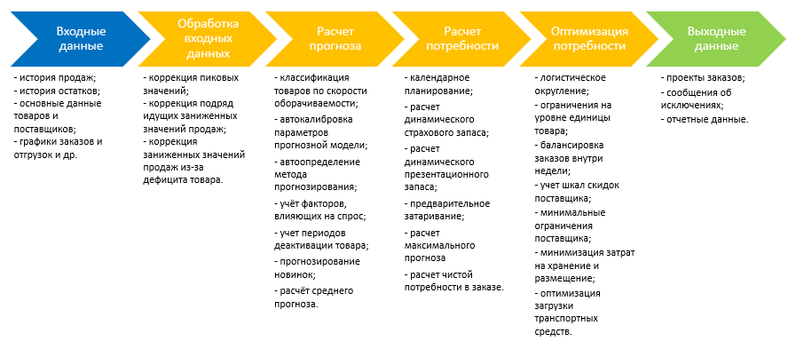
All the functionality of SAP F & R can be divided into 4 main blocks:
At the entrance to SAP F & R, sales data is presented in terms of product-location, history of balances, product and supplier master data, predefined delivery schedules and some tuning parameters that allow the system to function efficiently in accordance with the retailer's business.
It often happens that the sales statistics of the retailer is incorrect (unexplained peaks, lost days, underestimated sales due to the deficit are permissible). SAP F & R can work with inaccurate input data. The meaning of clearing statistics from outliers is to avoid the influence of outliers on the sales forecast. F & R first detects outliers and then replaces them with a local average of sales. The local average is the average between neighboring weeks, relative to the week with the extraneous value.
')
Example 1. Peak Correction
In the figure we see several unexplained system surges (peak sales). The black line is the real statistics, the red line is the adjusted sales values.
Detection: To detect extraneous values in the case of a peak, F & R calculates how strongly the value of weekly sales of peak or recession deviates from the local average weekly sales, taking into account neighboring weeks (two weeks on one side and two on the other). If the deviation from the local average> Standard deviation of the time series * coefficient, then such weekly sales are considered as extraneous values. The coefficient is set in the settings. Deviation from the local average = local average of weekly sales - the value of sales of a particular week, taken by module. The standard deviation of the time series is calculated for all weeks for which the sales history is provided.
Example 2. Correction of the history of undervalued due to the lack of sales data
The figure shows a clear wholesale sales of goods and, in consequence, zero stocks of goods or shortages. Days with a shortage of goods lead to incorrect sales statistics (lost sales are not counted). The system also corrects such values.
Discovery: Zero stock data is also uploaded to the system, as is input data. Products for which the stock was zero on some days of the week have undervalued sales for the week. The system adds to weekly sales a value = (Local average * number of days with a deficit per week) / number of working days per week.
Example 3. Correction of consecutive undervalued sales
The system also adjusts the sales history for too long consecutive periods of low weekly sales.
Detection: The detection length of consecutive weeks is set in the settings. If within a few weeks, where their number is not less than a given length, consecutive weekly sales are less than a specified threshold, then the system considers these weeks as weeks of underestimated sales and adjusts the sales history for these weeks in accordance with the local average.
In this block, the system predicts average sales values (or average forecast). The average forecast in the terminology of SAP F & R is such a value of the volume of goods on location, which with a probability of 50% will satisfy customer demand in the store, or, in other words, will ensure the level of customer service = 50%. The average forecast is not the end result put to the order.
To build an average forecast in the SAP F & R system, sales forecasting models are used, taking into account not only static consumption data, but also the influence of external factors, such as calendar events or promotions. The effect of such factors can be set either manually or automatically detected by the system in the past. Thus, when forming a predictive model of a time series, both in the past and in the future, SAP F & R uses data on a possible change in the predicted value and imposes the effect of an external factor on the smoothed series.
As can be seen in the figure, when forming a forecasting model in the past, SAP F & R clearly revealed seasonal sales fluctuations and peak spikes in the pre-New Year period and periods of other holidays.

As mentioned above, when calculating the average forecast, the system takes into account not only the sales behavior in the past, but also some features of the business. For a more flexible setting of the predictive model, all product-location combinations are divided into 6 groups according to the turnover rate: quick-turn 1, fast-turn 2, medium-turn 1, medium-turn 2, low-turn 1, low-turn 2. The boundaries of the values for which the distributions are made into groups are specified in the settings. Distribution by groups is a dynamic process, a product can belong to one group or to another in the case of an increase / decrease in turnover rate. Many business settings in the system are conducted in the context of these groups.
Also, on the basis of a group of products according to the speed of turnover in the system, the predictive model is automatically selected:
Methods can also be customized and manually at the request of the client company.
After selecting the prediction method, the system automatically calibrates the prediction model (calculation and selection of smoothing factors, trend, adaptability, etc., using the least prediction-fact error in the past).
Factors affecting demand
The system uses 3 main groups of factors affecting the demand:
Prediction of new products
In F & R, new items are predicted for 2 scenarios:
Example 4. Forecasting new products.
When specifying the counterpart from the same store, the sales history of the predecessor product is “glued” to the tail of the new product. The system predicts based on the statistics of sales of goods predecessor. There is no real sales history (black line). Red line: the history of the product analog.
Additional functionality
Also, SAP F & R can take into account periods of temporary exclusion of goods from the assortment matrix, the mutual influence of sales (when beer sales affect sales of chips, for example), using a reference module to predict sales of new products (combining the sales history of several goods), etc. etc. to achieve the most accurate result.
As I already wrote above, as a result of the module’s work, an average forecast is formed - such a value of the product’s volume on location, which with a probability of 50% will satisfy the demand of customers in the store, or, in other words, will ensure the level of customer service = 50%.
In order to avoid lost sales, the target level of customer service, as a rule, is planned to be not lower than 95%. This means that in 95 cases out of 100 the customer will buy what he planned in the store. Ensuring a high level of service in SAP F & R is made by means of an insurance premium to the average forecast, which depends not only on the target level of service, but also on the variability of past values of sales of goods. Thus, a maximum sales forecast is formed in the system, the volume of which will be sufficient to minimize stock in a warehouse or in a store (and, therefore, withdraw frozen capital in stocks) and meet the target level of customer service.
In the second part I will tell about the calculation of the need and optimization of the quantity of goods in the order.
Read my SAP F & R publications:
» Overview: SAP F & R today and tomorrow is the future of sales forecasting
»The Art of Forecasting in the SAP F & R System for Inventory Management
I remind you that SAP F & R is a demand forecasting and inventory management system at the level of target location-location provider. The system is part of the SAP SCM (Supply Chain Management) solution and is implemented in two variations:
- SAP F & R SCM - implementation with seamless integration with SAP systems;
- SAP F & R OI - system for integration with non-SAP systems.
All the functionality of SAP F & R can be divided into 4 main blocks:
- Input processing
- Forecast calculation
- Requirement calculation
- Needs optimization
At the entrance to SAP F & R, sales data is presented in terms of product-location, history of balances, product and supplier master data, predefined delivery schedules and some tuning parameters that allow the system to function efficiently in accordance with the retailer's business.
Input processing
It often happens that the sales statistics of the retailer is incorrect (unexplained peaks, lost days, underestimated sales due to the deficit are permissible). SAP F & R can work with inaccurate input data. The meaning of clearing statistics from outliers is to avoid the influence of outliers on the sales forecast. F & R first detects outliers and then replaces them with a local average of sales. The local average is the average between neighboring weeks, relative to the week with the extraneous value.
')
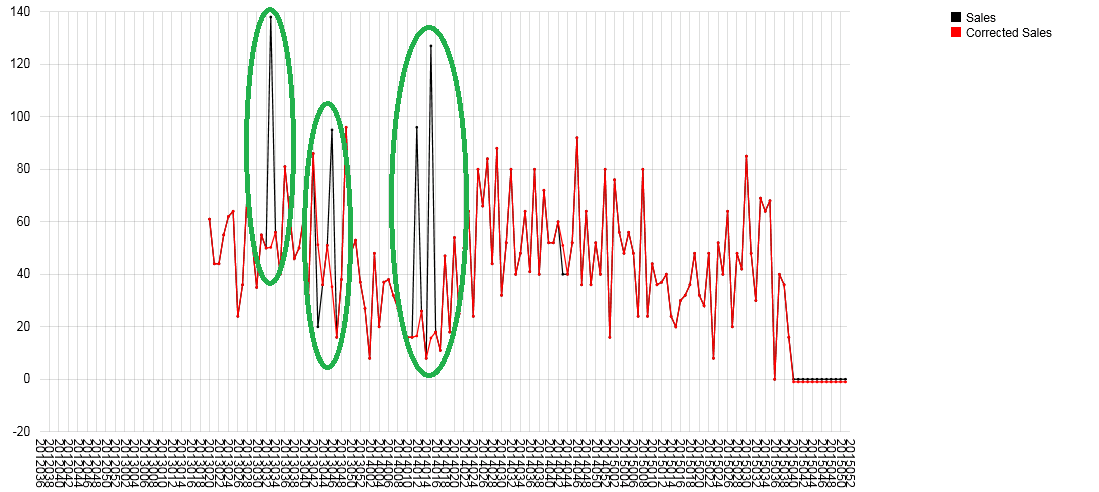
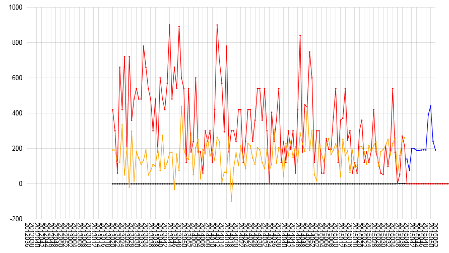
Example 1. Peak Correction
In the figure we see several unexplained system surges (peak sales). The black line is the real statistics, the red line is the adjusted sales values.
Detection: To detect extraneous values in the case of a peak, F & R calculates how strongly the value of weekly sales of peak or recession deviates from the local average weekly sales, taking into account neighboring weeks (two weeks on one side and two on the other). If the deviation from the local average> Standard deviation of the time series * coefficient, then such weekly sales are considered as extraneous values. The coefficient is set in the settings. Deviation from the local average = local average of weekly sales - the value of sales of a particular week, taken by module. The standard deviation of the time series is calculated for all weeks for which the sales history is provided.
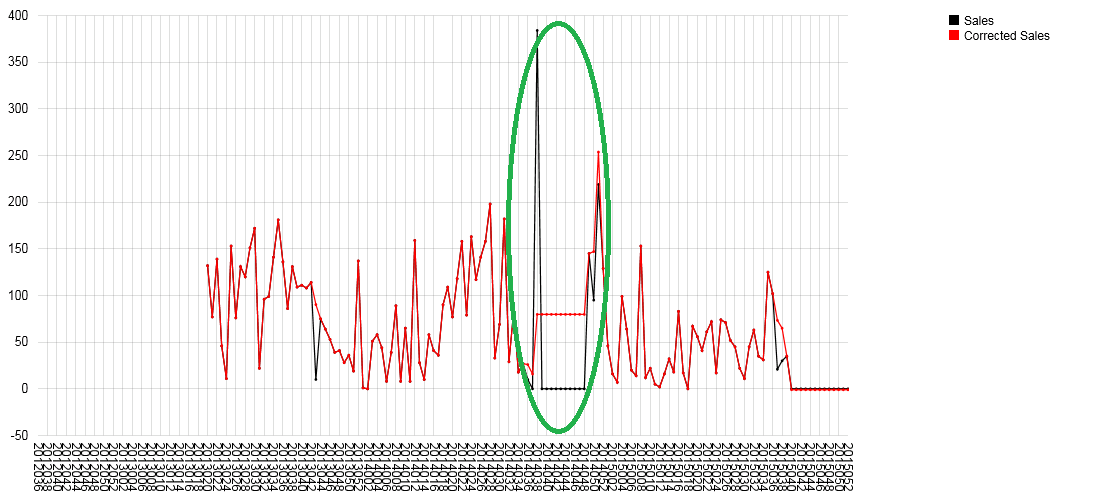
Example 2. Correction of the history of undervalued due to the lack of sales data
The figure shows a clear wholesale sales of goods and, in consequence, zero stocks of goods or shortages. Days with a shortage of goods lead to incorrect sales statistics (lost sales are not counted). The system also corrects such values.
Discovery: Zero stock data is also uploaded to the system, as is input data. Products for which the stock was zero on some days of the week have undervalued sales for the week. The system adds to weekly sales a value = (Local average * number of days with a deficit per week) / number of working days per week.
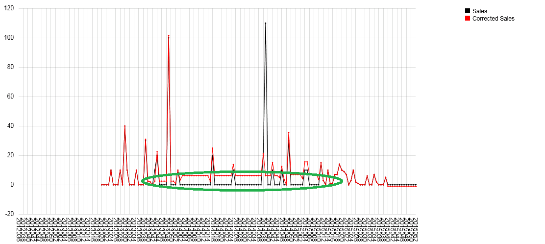
Example 3. Correction of consecutive undervalued sales
The system also adjusts the sales history for too long consecutive periods of low weekly sales.
Detection: The detection length of consecutive weeks is set in the settings. If within a few weeks, where their number is not less than a given length, consecutive weekly sales are less than a specified threshold, then the system considers these weeks as weeks of underestimated sales and adjusts the sales history for these weeks in accordance with the local average.
Forecast calculation
In this block, the system predicts average sales values (or average forecast). The average forecast in the terminology of SAP F & R is such a value of the volume of goods on location, which with a probability of 50% will satisfy customer demand in the store, or, in other words, will ensure the level of customer service = 50%. The average forecast is not the end result put to the order.
To build an average forecast in the SAP F & R system, sales forecasting models are used, taking into account not only static consumption data, but also the influence of external factors, such as calendar events or promotions. The effect of such factors can be set either manually or automatically detected by the system in the past. Thus, when forming a predictive model of a time series, both in the past and in the future, SAP F & R uses data on a possible change in the predicted value and imposes the effect of an external factor on the smoothed series.
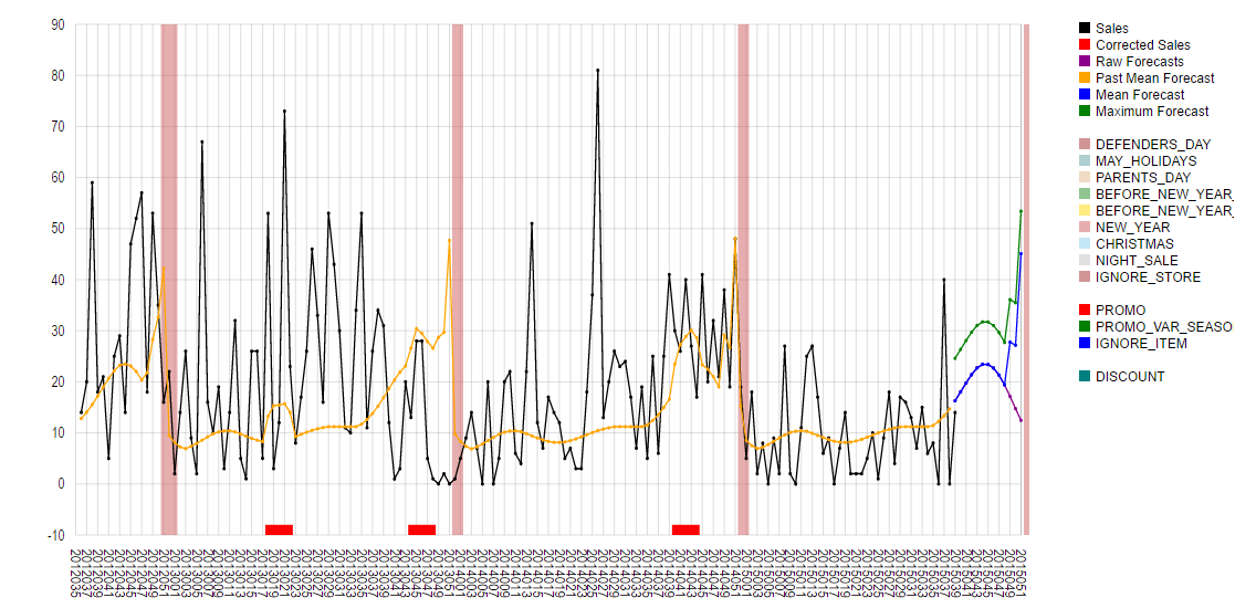
As can be seen in the figure, when forming a forecasting model in the past, SAP F & R clearly revealed seasonal sales fluctuations and peak spikes in the pre-New Year period and periods of other holidays.
As mentioned above, when calculating the average forecast, the system takes into account not only the sales behavior in the past, but also some features of the business. For a more flexible setting of the predictive model, all product-location combinations are divided into 6 groups according to the turnover rate: quick-turn 1, fast-turn 2, medium-turn 1, medium-turn 2, low-turn 1, low-turn 2. The boundaries of the values for which the distributions are made into groups are specified in the settings. Distribution by groups is a dynamic process, a product can belong to one group or to another in the case of an increase / decrease in turnover rate. Many business settings in the system are conducted in the context of these groups.
Also, on the basis of a group of products according to the speed of turnover in the system, the predictive model is automatically selected:
- Simplified forecasting methods (moving average, weighted average, etc.) are selected for new products whose sales history does not exceed 6 weeks.
- Constant methods (forecast = n) are used for products with a low turnover rate.
- Methods based on exponential smoothing and regression analysis are applied to all products, in the case of an external factor affecting sales, affecting demand.
Methods can also be customized and manually at the request of the client company.
After selecting the prediction method, the system automatically calibrates the prediction model (calculation and selection of smoothing factors, trend, adaptability, etc., using the least prediction-fact error in the past).
Factors affecting demand
The system uses 3 main groups of factors affecting the demand:
- Boolean factors: an event of a boolean factor consists of two possible situations: the factor is either valid or not (for example, promotional events, holidays, other calendar events). F & R assesses the effect on sales of goods on a store that was in the past due to an event factor, for example, a lifting factor equal to 1.5 caused by a promotion. If a factor event with the same indicator occurs in the future for the same product and store, the system will calculate its expected effect on the forecast. The figure shows the effect of PROMO factors, and the new year (+ weeks before the new year). The reaction to other factors is not so obvious. The forecast (blue line) is considered taking into account the action of the “Before the New Year” factor.
- Metric factors: a factor has a certain value at any given time (for example, price dynamics). The system evaluates the correlation between sales values under the action of a factor and the history of the consumption of goods. If a discount is used as a metric FCF, then during periods of non-rebate, the value of the FCF should be determined and equal to 0.
- Factor “Ignore”: events of this factor are used to exclude some periods of sales history from statistics, as they are not the correct values (for example, the period of repair of a part of a store, etc.).
Prediction of new products
In F & R, new items are predicted for 2 scenarios:
- Simplified: manual order or forecast using average methods to retrieve the required product history;
- Complicated: indication of the product predecessor from the same store.
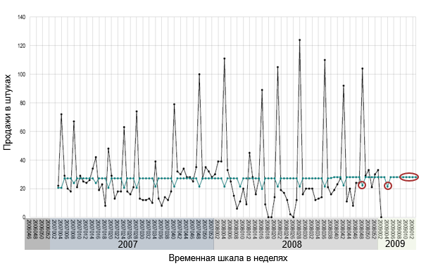
Example 4. Forecasting new products.
When specifying the counterpart from the same store, the sales history of the predecessor product is “glued” to the tail of the new product. The system predicts based on the statistics of sales of goods predecessor. There is no real sales history (black line). Red line: the history of the product analog.
Additional functionality
Also, SAP F & R can take into account periods of temporary exclusion of goods from the assortment matrix, the mutual influence of sales (when beer sales affect sales of chips, for example), using a reference module to predict sales of new products (combining the sales history of several goods), etc. etc. to achieve the most accurate result.
As I already wrote above, as a result of the module’s work, an average forecast is formed - such a value of the product’s volume on location, which with a probability of 50% will satisfy the demand of customers in the store, or, in other words, will ensure the level of customer service = 50%.
In order to avoid lost sales, the target level of customer service, as a rule, is planned to be not lower than 95%. This means that in 95 cases out of 100 the customer will buy what he planned in the store. Ensuring a high level of service in SAP F & R is made by means of an insurance premium to the average forecast, which depends not only on the target level of service, but also on the variability of past values of sales of goods. Thus, a maximum sales forecast is formed in the system, the volume of which will be sufficient to minimize stock in a warehouse or in a store (and, therefore, withdraw frozen capital in stocks) and meet the target level of customer service.
In the second part I will tell about the calculation of the need and optimization of the quantity of goods in the order.
Read my SAP F & R publications:
» Overview: SAP F & R today and tomorrow is the future of sales forecasting
»The Art of Forecasting in the SAP F & R System for Inventory Management
Source: https://habr.com/ru/post/308412/
All Articles