Simulation of dynamic systems (Lagrange method and Bond graph approach)
Good day to all. In this article I want to show one of the graphical methods for constructing mathematical models for dynamic systems, which is called Bond graph ("bond" - connections, "graph" - graph). In Russian literature, descriptions of this method, I found only in the textbook of Tomsk Polytechnic University, A.V. Voronin “MODELING OF MECHATRONIC SYSTEMS” 2008. Also show the classical method through the Lagrange equation of the 2nd kind.

I will not paint the theory, I will show the stages of calculations and with a few comments. Personally, I find it easier to learn by example than to read a theory 10 times. As it seemed to me, in Russian literature, the explanation of this method, and indeed of mathematics or physics, is very saturated with complex formulas, which therefore requires a serious mathematical background. While studying the Lagrange method (I study at the Turin Polytechnic University, Italy), I studied Russian literature to compare calculation methods, and it was hard for me to follow the course of solving this method. Even recalling the modeling courses at the Kharkiv Aviation Institute, the conclusion of such methods was very cumbersome, and no one made it difficult to try to sort out this issue. That's what I decided to write, a training manual for constructing mat models according to Lagrange, as it turned out this is not at all difficult, it is enough to know how to calculate time derivatives and partial derivatives. For models, it is even harder to add rotation matrices, but there is nothing complicated in them either.
Features of modeling methods:
')
Let's start with a simple example. Mass with spring and damper. Neglecting gravity.
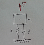
Figure 1 . Weight with spring and damper
First, we denote:
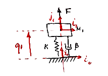
Figure 2 . We put down the coordinate systems and generalized coordinates
Next we find the position and velocity of all bodies. In this example, one body is M1:
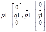
Figure 3 . Body position and speed M1
After we find the kinetic (C) and potential (P) energy and dissipative function (D) for the damper by the formulas:
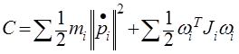
Figure 4 . Complete kinetic energy formula
In our example, there is no rotation, the second component is 0.
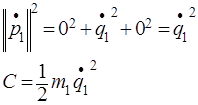

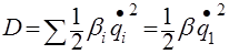
Figure 5 . Calculation of kinetic, potential energy and dissipative function
The Lagrange equation has the following form:

Figure 6 . Lagrange and Lagrangian equation
Delta W_i is a virtual work done by applied forces and moments. Find her:
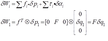
Figure 7 . Calculation of virtual work
where delta q_1 is the virtual displacement.
We substitute everything into the Lagrange equation:

Figure 8 . The resulting mass model with spring and damper
At this Lagrange method is over. As you can see, it is not so difficult, but it is still a very simple example, for which, most likely, the Newton-Euler method would even be simpler. For more complex systems, where there will be several bodies rotated relative to each other at different angles, the Lagrange method will be easier.
Immediately I will show the model in bond-graph as an example with a mass spring and a damper:
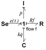
Figure 9 . Bond-graph mass with spring and damper
Here you have to tell a little theory, which is enough to build simple models. If anyone is interested, you can read a book ( [Wolfgang Borutzky] Bond Graph Methodology ) or ( Voronin AV, Modeling Mechatronic Systems: A Tutorial. - Tomsk: Tomsk Polytechnic University Publishing House, 2008 ).
To begin with, we define that complex systems consist of several domains. For example, an electric motor consists of electrical and mechanical parts or domains.
Bond graph is based on the exchange of power between these domains, subsystems. Note that the exchange of power, of any form, is always determined by two variables ( variable powers ) with the help of which we can study the interaction of different subsystems in the dynamic system (see table).
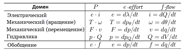
As can be seen from the table, the expression of power is almost the same everywhere. In a generalization, Power is the product of “ flow-f ” to “ effort-e ”.
The force (eng. Effort ) in the electric domain is voltage (e), in mechanical - force (F) or moment (T), in hydraulics - pressure (p).
The flow (English flow ) in the electrical domain is the current (i), in the mechanical domain - speed (v) or angular velocity (omega), in hydraulics - flow or fluid flow (Q).
Taking these designations, we obtain the expression for power:

Figure 10 . Formula of power through power variables
In the language of bond-graph, the connection between two subsystems that exchange power is represented by a bond (eng. Bond ). For this reason, this method is called bond-graph or g of raf-links, a connected graph . Consider the block diagram of connections in a model with an electric motor (this is not yet a bond graph):
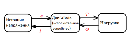
Figure 11 . Block diarama power flow between domains
If we have a voltage source, respectively, it generates voltage and gives it to the motor on the windings (the arrow points in the direction of the motor), depending on the winding resistance, a current appears according to Ohm's law (directed from the motor to the source). Accordingly, one variable is the input to the subsystem, and the second must be the output from the subsystem. Here the voltage ( effort ) is the input, the current ( flow ) is the output.
If you use a current source, how will the diagram change? Right. The current will be directed to the motor, and the voltage to the source. Then the current ( flow ) - input, voltage ( effort ) - output.
Consider an example in mechanics. The force acting on the mass.
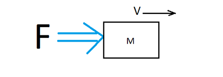
Figure 12 . Force applied to the mass
The block diagram will be as follows:
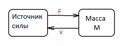
Figure 13 . Block diagram
In this example, Strength ( effort ) is the input variable for mass. (Force applied to mass)
According to Newton's second law:

Mass responds with speed:
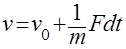
In this example, if one variable ( force — effort ) is the entrance to a mechanical domain, then the other power variable ( speed — flow ) automatically becomes an output .
To distinguish where the input is, and where the output is, a vertical line is used at the end of the arrow (connection) between the elements, this line is called the sign of causality or causality . It turns out: the applied force is the cause, and the speed is the effect. This sign is very important for the correct construction of the system model, since causality is a consequence of physical behavior and power exchange between the two subsystems, so the choice of the location of the causality sign cannot be arbitrary.
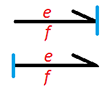
Figure 14 . Designation of causality
This vertical line shows which subsystem receives the effort ( effort ) and, as a result, produces a flow. In the example with the mass will be like this:
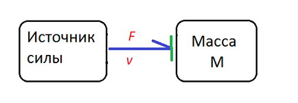
Figure 14 . Causal link for force acting on mass
In the direction of the arrow it is clear that the input for the mass is force , and the output is speed . This is done so as not to obstruct the scheme and systematize the construction of the model with arrows.
The next important point. Generalized impulse (amount of movement) and displacement ( energy variables ).
The table above introduces two additional physical quantities used in the bond-graph method. They are called the generalized momentum ( p ) and the generalized displacement ( q ) or energy variables, and they can be obtained by integrating the power variables over time:
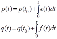
Figure 15 . The relationship between power and energy variables
In the electric domain :
Based on the Faraday law, the voltage at the ends of the conductor is equal to the derivative of the magnetic flux through this conductor.
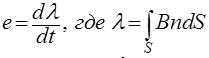
And the current strength is a physical quantity equal to the ratio of the amount of charge Q that has passed over time t through the conductor cross-section to the value of this period of time.

Mechanical Domain:
Of 2 Newton's laws, Strength is the time derivative of momentum
And accordingly, the speed is the time derivative of the movement:

Summarize :

All elements in dynamic systems can be divided into bipolar and quadripolar components.
Consider bipolar components :
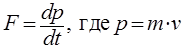
Sources
Sources are both effort and flow. Analogy in the electrical domain: the source of force is the source of voltage , the source of flow is the source of current . Causal signs for sources should be only such.
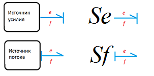
Figure 16 . Causal Relationship and Source Designation
Component R - dissipative element
Component I - inertial element
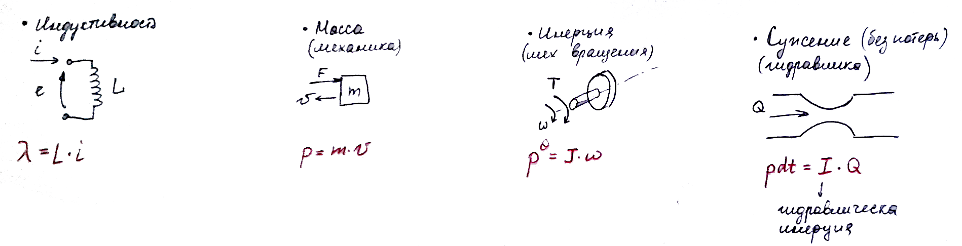
Component C - capacitive element
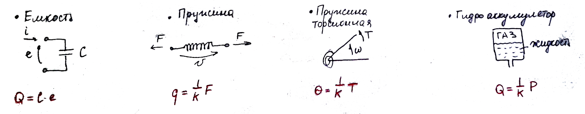
As can be seen from the figures, different elements of the same type of R, C, I are described by the same equations. ONLY there is a difference for electrical capacity, you just need to remember this!
Quadrupole components :
Consider the two components of the transformer and gyrator.
The last important components in the bond-graph method are connections. There are two types of nodes:
On it with components finished.
The main stages for affixing causal relationships after building a bond graph:
On this mini-course on the theory is over. Now we have everything you need to build models.
Let's solve a couple of examples. Let's start with the electrical circuit, better understand the analogy of constructing a bond graph.
The bottom line : for me, the bond-graph seemed more interesting. According to my observations, it is better to use it for complex systems (multi-domain systems, mechatronic systems). For example, AMESim , a powerful simulator of multi-domain systems, uses this method to build mat models. In robotics, the Lagrange method is likely to be easier. Who uses these methods, I will be glad to hear your conclusions, comments.
PS: link to course materials. (slides only on Lagrangian, on bond-graph - used mostly, a book and notes, which are only on paper)
Lagrange method
I will not paint the theory, I will show the stages of calculations and with a few comments. Personally, I find it easier to learn by example than to read a theory 10 times. As it seemed to me, in Russian literature, the explanation of this method, and indeed of mathematics or physics, is very saturated with complex formulas, which therefore requires a serious mathematical background. While studying the Lagrange method (I study at the Turin Polytechnic University, Italy), I studied Russian literature to compare calculation methods, and it was hard for me to follow the course of solving this method. Even recalling the modeling courses at the Kharkiv Aviation Institute, the conclusion of such methods was very cumbersome, and no one made it difficult to try to sort out this issue. That's what I decided to write, a training manual for constructing mat models according to Lagrange, as it turned out this is not at all difficult, it is enough to know how to calculate time derivatives and partial derivatives. For models, it is even harder to add rotation matrices, but there is nothing complicated in them either.
Features of modeling methods:
')
- Newton-Euler : vector equations based on dynamic equilibrium of forces (force) and moments (moments)
- Lagrange : scalar equations based on state functions related to kinetic and potential energy (energies)
- Bond-graph : a method based on the flow of power between the elements of the system
Let's start with a simple example. Mass with spring and damper. Neglecting gravity.
Figure 1 . Weight with spring and damper
First, we denote:
- the initial coordinate system (NSC) or stationary sk R0 (i0, j0, k0) . Where? You can poke your finger into the sky, but by pulling the tips of neurons in the brain, the idea is to put the NSC on the line of motion of the body M1.
- coordinate systems for each body with mass (we have M1 R1 (i1, j1, k1) ), the orientation can be arbitrary, but why complicate our lives, set with minimal difference from the NSC
- generalized coordinates q_i (the minimum number of variables that can describe the movement), in this example, one generalized coordinate, movement only along the j axis
Figure 2 . We put down the coordinate systems and generalized coordinates
Next we find the position and velocity of all bodies. In this example, one body is M1:
Figure 3 . Body position and speed M1
After we find the kinetic (C) and potential (P) energy and dissipative function (D) for the damper by the formulas:
Figure 4 . Complete kinetic energy formula
In our example, there is no rotation, the second component is 0.
Figure 5 . Calculation of kinetic, potential energy and dissipative function
The Lagrange equation has the following form:
Figure 6 . Lagrange and Lagrangian equation
Delta W_i is a virtual work done by applied forces and moments. Find her:
Figure 7 . Calculation of virtual work
where delta q_1 is the virtual displacement.
We substitute everything into the Lagrange equation:
Figure 8 . The resulting mass model with spring and damper
At this Lagrange method is over. As you can see, it is not so difficult, but it is still a very simple example, for which, most likely, the Newton-Euler method would even be simpler. For more complex systems, where there will be several bodies rotated relative to each other at different angles, the Lagrange method will be easier.
Bond graph method
Immediately I will show the model in bond-graph as an example with a mass spring and a damper:
Figure 9 . Bond-graph mass with spring and damper
Here you have to tell a little theory, which is enough to build simple models. If anyone is interested, you can read a book ( [Wolfgang Borutzky] Bond Graph Methodology ) or ( Voronin AV, Modeling Mechatronic Systems: A Tutorial. - Tomsk: Tomsk Polytechnic University Publishing House, 2008 ).
To begin with, we define that complex systems consist of several domains. For example, an electric motor consists of electrical and mechanical parts or domains.
Bond graph is based on the exchange of power between these domains, subsystems. Note that the exchange of power, of any form, is always determined by two variables ( variable powers ) with the help of which we can study the interaction of different subsystems in the dynamic system (see table).
As can be seen from the table, the expression of power is almost the same everywhere. In a generalization, Power is the product of “ flow-f ” to “ effort-e ”.
The force (eng. Effort ) in the electric domain is voltage (e), in mechanical - force (F) or moment (T), in hydraulics - pressure (p).
The flow (English flow ) in the electrical domain is the current (i), in the mechanical domain - speed (v) or angular velocity (omega), in hydraulics - flow or fluid flow (Q).
Taking these designations, we obtain the expression for power:
Figure 10 . Formula of power through power variables
In the language of bond-graph, the connection between two subsystems that exchange power is represented by a bond (eng. Bond ). For this reason, this method is called bond-graph or g of raf-links, a connected graph . Consider the block diagram of connections in a model with an electric motor (this is not yet a bond graph):
Figure 11 . Block diarama power flow between domains
If we have a voltage source, respectively, it generates voltage and gives it to the motor on the windings (the arrow points in the direction of the motor), depending on the winding resistance, a current appears according to Ohm's law (directed from the motor to the source). Accordingly, one variable is the input to the subsystem, and the second must be the output from the subsystem. Here the voltage ( effort ) is the input, the current ( flow ) is the output.
If you use a current source, how will the diagram change? Right. The current will be directed to the motor, and the voltage to the source. Then the current ( flow ) - input, voltage ( effort ) - output.
Consider an example in mechanics. The force acting on the mass.
Figure 12 . Force applied to the mass
The block diagram will be as follows:
Figure 13 . Block diagram
In this example, Strength ( effort ) is the input variable for mass. (Force applied to mass)
According to Newton's second law:
Mass responds with speed:
In this example, if one variable ( force — effort ) is the entrance to a mechanical domain, then the other power variable ( speed — flow ) automatically becomes an output .
To distinguish where the input is, and where the output is, a vertical line is used at the end of the arrow (connection) between the elements, this line is called the sign of causality or causality . It turns out: the applied force is the cause, and the speed is the effect. This sign is very important for the correct construction of the system model, since causality is a consequence of physical behavior and power exchange between the two subsystems, so the choice of the location of the causality sign cannot be arbitrary.
Figure 14 . Designation of causality
This vertical line shows which subsystem receives the effort ( effort ) and, as a result, produces a flow. In the example with the mass will be like this:
Figure 14 . Causal link for force acting on mass
In the direction of the arrow it is clear that the input for the mass is force , and the output is speed . This is done so as not to obstruct the scheme and systematize the construction of the model with arrows.
The next important point. Generalized impulse (amount of movement) and displacement ( energy variables ).
Table of power and energy variables in different domains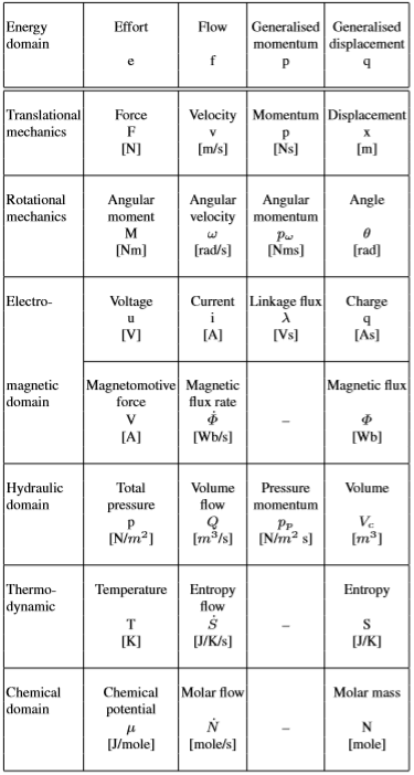
The table above introduces two additional physical quantities used in the bond-graph method. They are called the generalized momentum ( p ) and the generalized displacement ( q ) or energy variables, and they can be obtained by integrating the power variables over time:
Figure 15 . The relationship between power and energy variables
In the electric domain :
Based on the Faraday law, the voltage at the ends of the conductor is equal to the derivative of the magnetic flux through this conductor.
And the current strength is a physical quantity equal to the ratio of the amount of charge Q that has passed over time t through the conductor cross-section to the value of this period of time.
Mechanical Domain:
Of 2 Newton's laws, Strength is the time derivative of momentum
And accordingly, the speed is the time derivative of the movement:
Summarize :
Basic elements
All elements in dynamic systems can be divided into bipolar and quadripolar components.
Consider bipolar components :
Sources
Sources are both effort and flow. Analogy in the electrical domain: the source of force is the source of voltage , the source of flow is the source of current . Causal signs for sources should be only such.
Figure 16 . Causal Relationship and Source Designation
Component R - dissipative element
Component I - inertial element
Component C - capacitive element
As can be seen from the figures, different elements of the same type of R, C, I are described by the same equations. ONLY there is a difference for electrical capacity, you just need to remember this!
Quadrupole components :
Consider the two components of the transformer and gyrator.
- Ideal Transformer (TF) connects values of the same type between the input and the output
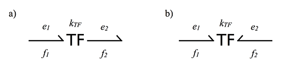
Formulas describing the transformer from figure a and b, respectively: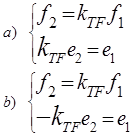
Causal signs are placed only as shown below.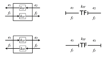
This is not so: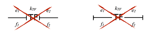 Examples of a transformer in a mechanical domain can be a gear drive, a lever
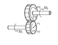

An ordinary transformer is in electricity. Hydraulic piston - in hydraulics. - Gyrator (GY). The ideal Gyrator binds the flow on one side with the effort on the other.
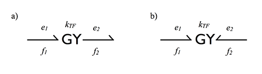
Formulas:
Allowable causality for gyrator: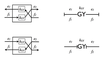
Erroneous causality: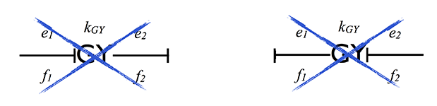
Examples of gyrators: in mechanics this is a dc motor, in electronics it is a solenoid (linear actuator).
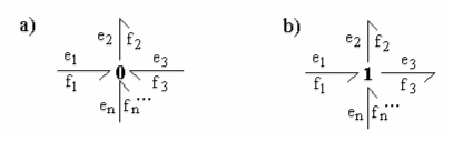
The last important components in the bond-graph method are connections. There are two types of nodes:
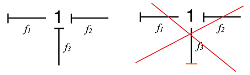
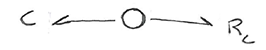
- Node type 0 (a) - they have a common effort and only one causal link must enter the 0-node, the rest must go out.
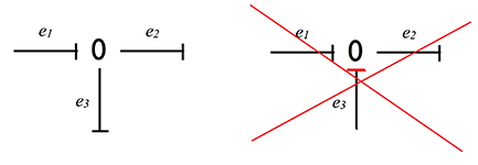
Consider an example of a 0-node calculation: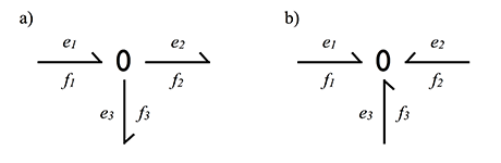
a) 0 means all efforts are equal
Since the node does not accumulate and does not dissipate energy, then the algebraic sum of the incoming power must be zero.
Considering the previous equation we get
b) For the second option we get
- Node type 1 (b) - they have a common flow and only one causal link should go out, the rest should go into a 1-node.
Consider the calculation of 1-node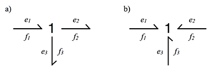
a) 1 node has a common flow, it means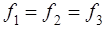
Since the node does not accumulate and does not dissipate energy, then the algebraic sum of the incoming power must be zero.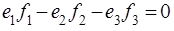
Given the previous equation we get: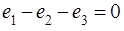
b) Here will be:
On it with components finished.
The main stages for affixing causal relationships after building a bond graph:
- Make causal links to all sources
- Go through all the nodes and put down causal relationships after point 1
- For components I, assign an input causal relationship (force enters this component), for components C, assign an output causal relationship (force leaves this component)
- Repeat point 2
- Put causal relationships for the components of R
On this mini-course on the theory is over. Now we have everything you need to build models.
Let's solve a couple of examples. Let's start with the electrical circuit, better understand the analogy of constructing a bond graph.
Example 1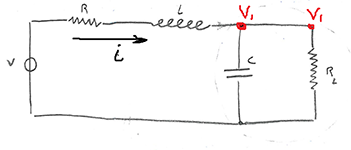
Let's start building a bond graph with a voltage source. Just write Se and put the arrow.

See all easy! We look further, R and L are connected in series, meaning the same current flows in them, if we talk in power variables - the same flow. Which node has the same flow? The correct answer is 1-node. Connect to 1-node source, resistance (component - R) and inductance (component - I).
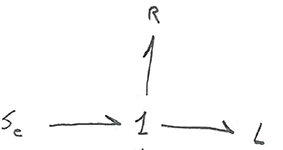
Next we have the capacitance and resistance in parallel, which means they have the same voltage or force. 0-node is suitable like no other. We connect the capacitance (component C) and the resistance (component R) to the 0-node.
Nodes 1 and 0 are also connected to each other. The direction of the arrows is arbitrary, the direction of the connection affects only the sign in the equations.
Get the following link graph:

Now you need to put down a causal relationship. Following the instructions on the sequence of their affixing, let's start with the source.
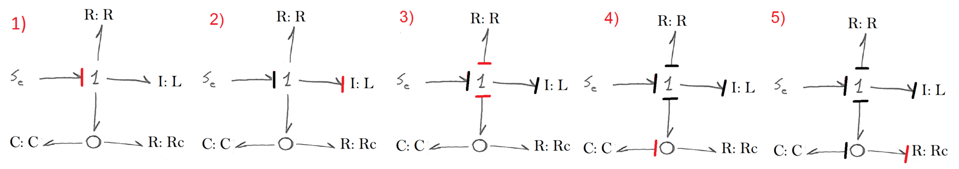
That's all. Bond-graph built. Cheers, Comrades!
It remains the case for small, write the equations describing our system. To do this, create a table with 3 columns. In the first there will be all the components of the system, in the second there will be an input variable for each element, and in the third - an output variable for the same component. We have already defined the entrance and exit by causal relationships. So there should be no problems.
Let us number each link for the convenience of writing equations. Equations for each element are taken from the list of components C, R, I.
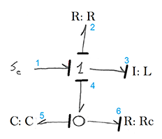
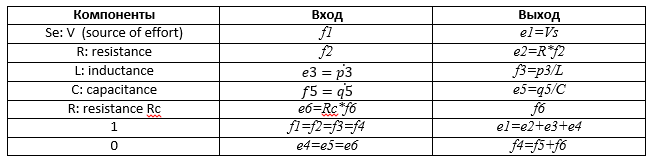
Making a table, we define state variables; in this example, they are 2, p3 and q5. Next you need to write the equations of state:
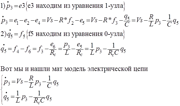
That's all the model is ready.
Let's start building a bond graph with a voltage source. Just write Se and put the arrow.
See all easy! We look further, R and L are connected in series, meaning the same current flows in them, if we talk in power variables - the same flow. Which node has the same flow? The correct answer is 1-node. Connect to 1-node source, resistance (component - R) and inductance (component - I).
Next we have the capacitance and resistance in parallel, which means they have the same voltage or force. 0-node is suitable like no other. We connect the capacitance (component C) and the resistance (component R) to the 0-node.
Nodes 1 and 0 are also connected to each other. The direction of the arrows is arbitrary, the direction of the connection affects only the sign in the equations.
Get the following link graph:
Now you need to put down a causal relationship. Following the instructions on the sequence of their affixing, let's start with the source.
- We have a source of tension (effort), such a source has only one variant of causality - the output. We put.
- Next is the component I, look what is recommended. We put
- We put down for 1-node. there is
- A 0-node must have one input and all output causal relationships. We still have one day off. We are looking for components C or I. Found. We put
- We put down what's left
That's all. Bond-graph built. Cheers, Comrades!
It remains the case for small, write the equations describing our system. To do this, create a table with 3 columns. In the first there will be all the components of the system, in the second there will be an input variable for each element, and in the third - an output variable for the same component. We have already defined the entrance and exit by causal relationships. So there should be no problems.
Let us number each link for the convenience of writing equations. Equations for each element are taken from the list of components C, R, I.
Making a table, we define state variables; in this example, they are 2, p3 and q5. Next you need to write the equations of state:
That's all the model is ready.
Example 2. I just want to apologize for the quality of the photo, the main thing that you can read
Let's solve one more example for the mechanical system, the same one that we solved by the Lagrange method. I will show the decision without comment. Let's check which of these methods is easier, easier.
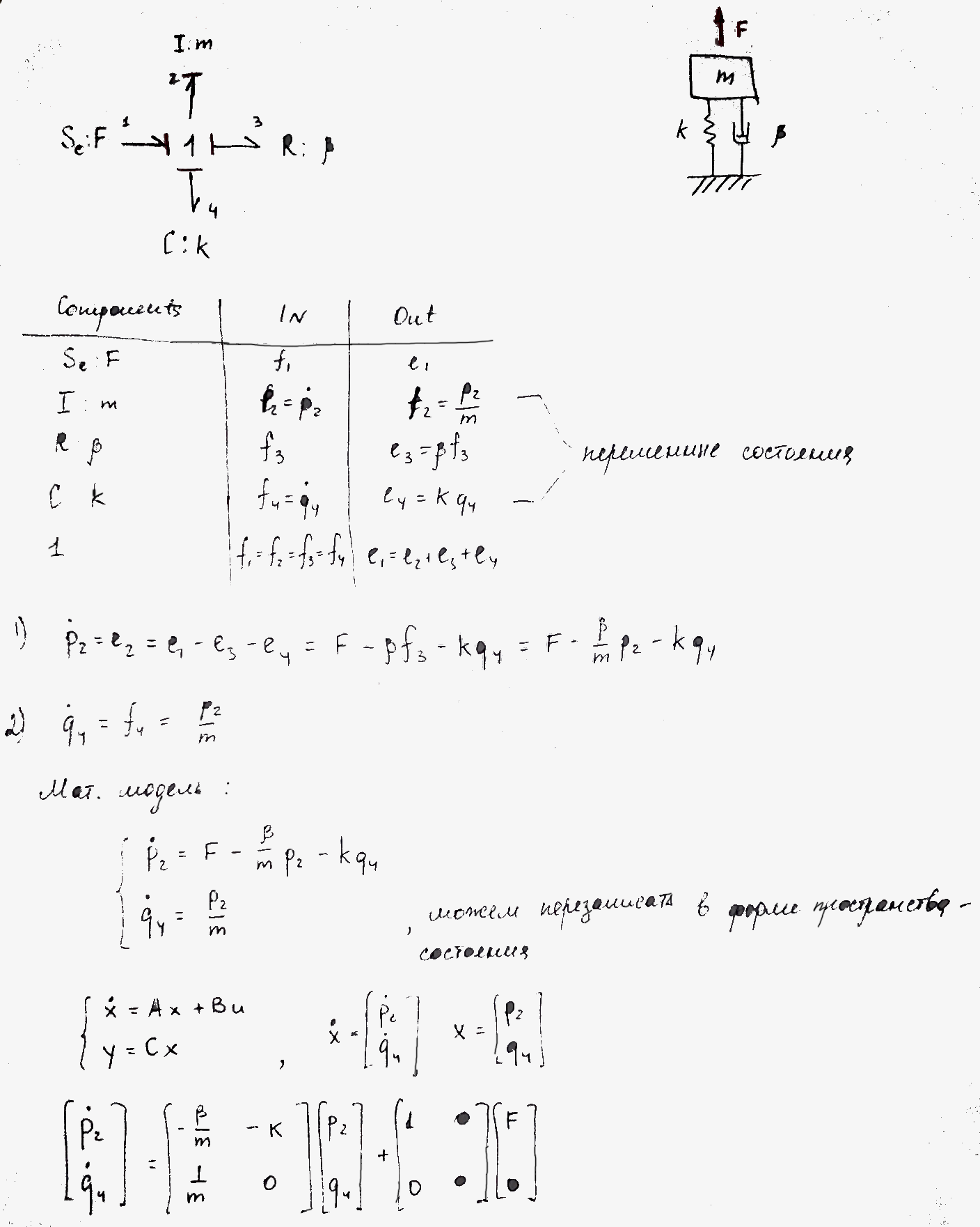
Both mat models with the same parameters, obtained by the Lagrange method and bond graph, were compiled in the matrix. Result below:
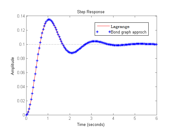
Both mat models with the same parameters, obtained by the Lagrange method and bond graph, were compiled in the matrix. Result below:
The bottom line : for me, the bond-graph seemed more interesting. According to my observations, it is better to use it for complex systems (multi-domain systems, mechatronic systems). For example, AMESim , a powerful simulator of multi-domain systems, uses this method to build mat models. In robotics, the Lagrange method is likely to be easier. Who uses these methods, I will be glad to hear your conclusions, comments.
PS: link to course materials. (slides only on Lagrangian, on bond-graph - used mostly, a book and notes, which are only on paper)
Source: https://habr.com/ru/post/307814/
All Articles