Mathematics for artificial neural networks for beginners, part 2 - gradient descent
Part 1 - linear regression
In the first part, I forgot to mention that if randomly generated data is not to your liking, then you can take any suitable example from here . You can feel like a nerd , winemaker , seller . And all this without getting up from the chair. In the presence of many data sets and one condition - when publishing, indicate where the data came from so that others could reproduce the results.
In the last part, an example of calculating linear regression parameters using the least squares method was shown. Parameters were found analytically - where
where  - pseudoinverse matrix. This solution is visual, accurate and short. But there is a problem that can be solved numerically. Gradient descent is a method of numerical optimization, which can be used in many algorithms where it is required to find the extremum of a function — neural networks, SVM, k-means, regression. However, it is easier to perceive in its pure form (and easier to modify).
The problem is that the calculation of the pseudoinverse is very expensive : 2 multiplications by , finding the inverse matrix - multiplying matrix vector
  where n is the number of elements in the matrix A (the number of attributes * the number of elements in the test sample) If the number of elements in matrix A is large (> 10 ^ 6 - for example), then even if there are 10,000 cores available, finding the solution can be analytically delayed. Also, the first derivative may be non-linear, which complicates the decision, the analytical solution may not be at all, or the data may simply not get into memory and an iterative algorithm will be required. It happens that they write down the advantages that the numerical solution is not ideally accurate. In this regard, the cost function is minimized by numerical methods. The task of finding the extremum is called the optimization problem. In this part I will focus on the optimization method, which is called gradient descent.
')
We will not deviate from linear regression and OLS and denote the loss function as
as 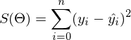 - it remained unchanged. Let me remind you that the gradient is a type vector
 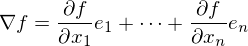 where
where  - This is a private derivative. One of the properties of the gradient is that it indicates the direction in which some function f increases the most. The proof of this follows from the definition of a derivative. A pair of evidence . Take some point a - in the vicinity of this point, the function F must be defined and differentiable, then the anti-gradient vector will indicate the direction in which the function F decreases the fastest. From here it is concluded that at some point b, equal to
 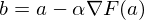 with some small
  the value of the function will be less than or equal to the value at point a. You can imagine this as a movement down the hill - taking a step down, the current position will be lower than the previous one. Thus, at each next step, the height will at least not increase. Formal definition . Based on these definitions, you can get a formula for finding unknown parameters (this is just a rewritten version of the formula above):
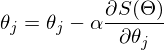
- this is a step of the method. In machine learning tasks, it is called learning speed.
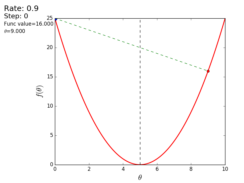
The method is very simple and intuitive, take a simple two-dimensional example to demonstrate:
It is necessary to minimize the function of the form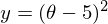 . Minimizing means finding at what value
  function
  takes the minimum value. We define the sequence of actions:
1) Derivative with respect to : 
2) Set the initial value = 0
3) Set the step size - try several values - 0.1, 0.9, 1.2, to see how this choice will affect the convergence.
4) 25 times in a row, execute the above formula: Since there is only one unknown parameter, there is only one formula.
The code is extremely simple. Excluding the definition of functions, the whole algorithm fit into 3 lines:
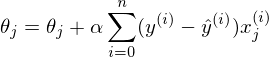
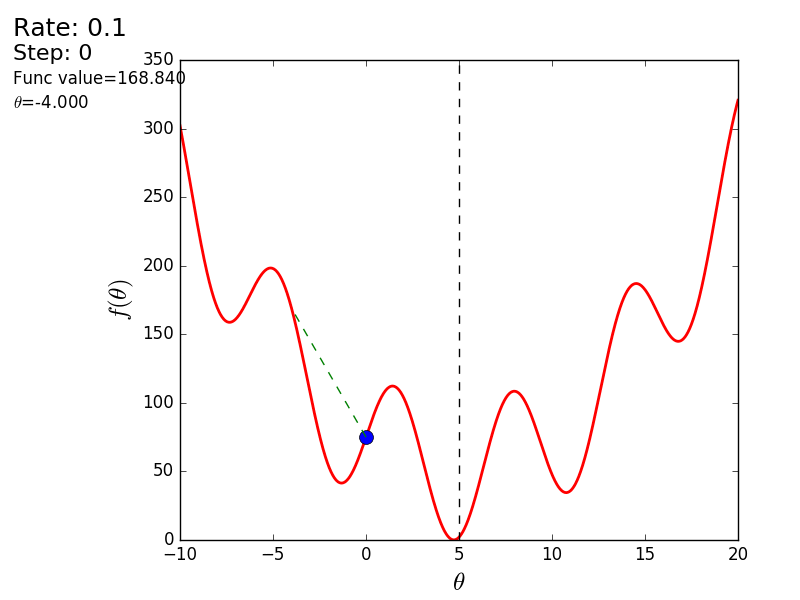
The whole process can be visualized in the following way (the blue dot is the value at the previous step, the red dot is the current one):
Or for a step of a different size:
With a value of 1.2, the method diverges, each step falling not lower, but vice versa higher, rushing to infinity. A step in a simple implementation is selected manually and its size depends on the data - on some unnormalized values with a large gradient and 0.0001 can lead to a discrepancy.
Here is another example of a “bad” function. In the first animation, the method also diverges and will wander for a long time over the hills due to a step too high. In the second case, a local minimum was found and, by varying the speed value, it would not work to force the method to find the minimum global. This fact is one of the drawbacks of the method - it can find a global minimum only if the function is convex and smooth. Or if you are lucky with the initial values.
It is also possible to consider the operation of the algorithm on three-dimensional graphics. Often draw only the isolines of a figure. I took a simple paraboloid of rotation: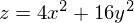 . In 3D, it looks like this:
  , and the graph with isolines is “top view”.
Also note that all the gradient lines are perpendicular to the isolines. This means that, moving towards the antigradient, it will not be possible to immediately jump to the minimum in one step - the gradient indicates not at all there.
After a graphic explanation, we find the formula for calculating the unknown parameters linear regression with OLS.
If the number of elements in the test sample were equal to one, then the formula could be left and considered. In the case when there are n elements, the algorithm looks like this:
Repeat v times
{
for each j at the same time.
}, where n is the number of elements in the training sample, v is the number of iterations
The requirement of simultaneity means that the derivative should be calculated with the old values of theta, you should not first calculate the first parameter, then the second, etc., because after changing the first parameter separately, the derivative will also change its value. Pseudo-code simultaneous change:
If we calculate the values of the parameters one by one, then this will no longer be a gradient descent. Suppose we have a three-dimensional figure, and if we calculate the parameters one by one, then we can think of this process as moving only one coordinate at a time — one small step along the x coordinate, then a step along the y coordinate, and so on. steps, instead of moving in the direction of the antigradient vector.
The above variant of the algorithm is called a packet gradient descent. The number of repetitions can be replaced by the phrase "Repeat until it converges." This phrase means that the parameters will be adjusted until the previous and current values of the cost function are equal. This means that a local or global minimum has been found and the algorithm will not go on. In practice, equality cannot be achieved and the limit of convergence is introduced. . It is established by some small value and the stopping criterion is that the difference between the previous and current values is less than the limit of convergence - this means that the minimum has been reached with the required accuracy. Higher accuracy (less ) - more iterations of the algorithm. It looks something like this:
Since the post suddenly stretched out, I would like to finish it on this - in the next part I will continue to analyze the gradient descent for linear regression with OLS.
Continued .
To run the examples you need: numpy, matplotlib.
ImageMagick is required to run examples that create animations.
The materials used in the article - github.com/m9psy/neural_network_habr_guide
In the first part, I forgot to mention that if randomly generated data is not to your liking, then you can take any suitable example from here . You can feel like a nerd , winemaker , seller . And all this without getting up from the chair. In the presence of many data sets and one condition - when publishing, indicate where the data came from so that others could reproduce the results.
Gradient descent
In the last part, an example of calculating linear regression parameters using the least squares method was shown. Parameters were found analytically -
where - pseudoinverse matrix. This solution is visual, accurate and short. But there is a problem that can be solved numerically. Gradient descent is a method of numerical optimization, which can be used in many algorithms where it is required to find the extremum of a function — neural networks, SVM, k-means, regression. However, it is easier to perceive in its pure form (and easier to modify).The problem is that the calculation of the pseudoinverse is very expensive : 2 multiplications by
, finding the inverse matrix - multiplying matrix vector where n is the number of elements in the matrix A (the number of attributes * the number of elements in the test sample) If the number of elements in matrix A is large (> 10 ^ 6 - for example), then even if there are 10,000 cores available, finding the solution can be analytically delayed. Also, the first derivative may be non-linear, which complicates the decision, the analytical solution may not be at all, or the data may simply not get into memory and an iterative algorithm will be required. It happens that they write down the advantages that the numerical solution is not ideally accurate. In this regard, the cost function is minimized by numerical methods. The task of finding the extremum is called the optimization problem. In this part I will focus on the optimization method, which is called gradient descent.')
We will not deviate from linear regression and OLS and denote the loss function
as - it remained unchanged. Let me remind you that the gradient is a type vector where - This is a private derivative. One of the properties of the gradient is that it indicates the direction in which some function f increases the most. The proof of this follows from the definition of a derivative. A pair of evidence . Take some point a - in the vicinity of this point, the function F must be defined and differentiable, then the anti-gradient vector will indicate the direction in which the function F decreases the fastest. From here it is concluded that at some point b, equal to with some small the value of the function will be less than or equal to the value at point a. You can imagine this as a movement down the hill - taking a step down, the current position will be lower than the previous one. Thus, at each next step, the height will at least not increase. Formal definition . Based on these definitions, you can get a formula for finding unknown parameters (this is just a rewritten version of the formula above): - this is a step of the method. In machine learning tasks, it is called learning speed.The method is very simple and intuitive, take a simple two-dimensional example to demonstrate:
It is necessary to minimize the function of the form
. Minimizing means finding at what value function takes the minimum value. We define the sequence of actions:1) Derivative with respect to
: 2) Set the initial value
= 03) Set the step size - try several values - 0.1, 0.9, 1.2, to see how this choice will affect the convergence.
4) 25 times in a row, execute the above formula:
Since there is only one unknown parameter, there is only one formula.The code is extremely simple. Excluding the definition of functions, the whole algorithm fit into 3 lines:
simple_gd_console.py
STEP_COUNT = 25 STEP_SIZE = 0.1 # def func(x): return (x - 5) ** 2 def func_derivative(x): return 2 * (x - 5) previous_x, current_x = 0, 0 for i in range(STEP_COUNT): current_x = previous_x - STEP_SIZE * func_derivative(previous_x) previous_x = current_x print("After", STEP_COUNT, "steps theta=", format(current_x, ".6f"), "function value=", format(func(current_x), ".6f")) The whole process can be visualized in the following way (the blue dot is the value at the previous step, the red dot is the current one):
Or for a step of a different size:
With a value of 1.2, the method diverges, each step falling not lower, but vice versa higher, rushing to infinity. A step in a simple implementation is selected manually and its size depends on the data - on some unnormalized values with a large gradient and 0.0001 can lead to a discrepancy.
Code for generating gifs
import matplotlib.pyplot as plt import matplotlib.animation as anim import numpy as np STEP_COUNT = 25 STEP_SIZE = 0.1 # X = [i for i in np.linspace(0, 10, 10000)] def func(x): return (x - 5) ** 2 def bad_func(x): return (x - 5) ** 2 + 50 * np.sin(x) + 50 Y = [func(x) for x in X] def func_derivative(x): return 2 * (x - 5) def bad_func_derivative(x): return 2 * (x + 25 * np.cos(x) - 5) # - skip_first = True def draw_gradient_points(num, points, line, cost_caption, step_caption, theta_caption): global previous_x, skip_first, ax if skip_first: skip_first = False return points, line current_x = previous_x - STEP_SIZE * func_derivative(previous_x) step_caption.set_text("Step: " + str(num)) cost_caption.set_text("Func value=" + format(func(current_x), ".3f")) theta_caption.set_text("$\\theta$=" + format(current_x, ".3f")) print("Step:", num, "Previous:", previous_x, "Current", current_x) points[0].set_data(previous_x, func(previous_x)) points[1].set_data(current_x, func(current_x)) # points.set_data([previous_x, current_x], [func(previous_x), func(current_x)]) line.set_data([previous_x, current_x], [func(previous_x), func(current_x)]) if np.abs(func(previous_x) - func(current_x)) < 0.5: ax.axis([4, 6, 0, 1]) if np.abs(func(previous_x) - func(current_x)) < 0.1: ax.axis([4.5, 5.5, 0, 0.5]) if np.abs(func(previous_x) - func(current_x)) < 0.01: ax.axis([4.9, 5.1, 0, 0.08]) previous_x = current_x return points, line previous_x = 0 fig, ax = plt.subplots() p = ax.get_position() ax.set_position([p.x0 + 0.1, p.y0, p.width * 0.9, p.height]) ax.set_xlabel("$\\theta$", fontsize=18) ax.set_ylabel("$f(\\theta)$", fontsize=18) ax.plot(X, Y, '-r', linewidth=2.0) ax.axvline(5, color='black', linestyle='--') start_point, = ax.plot([], 'bo', markersize=10.0) end_point, = ax.plot([], 'ro') rate_capt = ax.text(-0.3, 1.05, "Rate: " + str(STEP_SIZE), fontsize=18, transform=ax.transAxes) step_caption = ax.text(-0.3, 1, "Step: ", fontsize=16, transform=ax.transAxes) cost_caption = ax.text(-0.3, 0.95, "Func value: ", fontsize=12, transform=ax.transAxes) theta_caption = ax.text(-0.3, 0.9, "$\\theta$=", fontsize=12, transform=ax.transAxes) points = (start_point, end_point) line, = ax.plot([], 'g--') gradient_anim = anim.FuncAnimation(fig, draw_gradient_points, frames=STEP_COUNT, fargs=(points, line, cost_caption, step_caption, theta_caption), interval=1500) # , ImageMagick # .mp4 magick-shmagick gradient_anim.save("images/animation.gif", writer="imagemagick") Here is another example of a “bad” function. In the first animation, the method also diverges and will wander for a long time over the hills due to a step too high. In the second case, a local minimum was found and, by varying the speed value, it would not work to force the method to find the minimum global. This fact is one of the drawbacks of the method - it can find a global minimum only if the function is convex and smooth. Or if you are lucky with the initial values.
Bad function
Bad feature: 
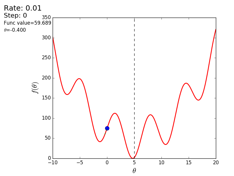
It is also possible to consider the operation of the algorithm on three-dimensional graphics. Often draw only the isolines of a figure. I took a simple paraboloid of rotation:
. In 3D, it looks like this: , and the graph with isolines is “top view”.Contour plot
Generating a graph with isolines
import matplotlib.pyplot as plt import matplotlib.animation as anim import numpy as np STEP_COUNT = 25 STEP_SIZE = 0.005 # X = np.array([i for i in np.linspace(-10, 10, 1000)]) Y = np.array([i for i in np.linspace(-10, 10, 1000)]) def func(X, Y): return 4 * (X ** 2) + 16 * (Y ** 2) def dx(x): return 8 * x def dy(y): return 32 * y # - skip_first = True def draw_gradient_points(num, point, line): global previous_x, previous_y, skip_first, ax if skip_first: skip_first = False return point current_x = previous_x - STEP_SIZE * dx(previous_x) current_y = previous_y - STEP_SIZE * dy(previous_y) print("Step:", num, "CurX:", current_x, "CurY", current_y, "Fun:", func(current_x, current_y)) point.set_data([current_x], [current_y]) # Blah-blah new_x = list(line.get_xdata()) + [previous_x, current_x] new_y = list(line.get_ydata()) + [previous_y, current_y] line.set_xdata(new_x) line.set_ydata(new_y) previous_x = current_x previous_y = current_y return point previous_x, previous_y = 8.8, 8.5 fig, ax = plt.subplots() p = ax.get_position() ax.set_position([p.x0 + 0.1, p.y0, p.width * 0.9, p.height]) ax.set_xlabel("X", fontsize=18) ax.set_ylabel("Y", fontsize=18) X, Y = np.meshgrid(X, Y) plt.contour(X, Y, func(X, Y)) point, = plt.plot([8.8], [8.5], 'bo') line, = plt.plot([], color='black') gradient_anim = anim.FuncAnimation(fig, draw_gradient_points, frames=STEP_COUNT, fargs=(point, line), interval=1500) # , ImageMagick # .mp4 magick-shmagick gradient_anim.save("images/contour_plot.gif", writer="imagemagick") Also note that all the gradient lines are perpendicular to the isolines. This means that, moving towards the antigradient, it will not be possible to immediately jump to the minimum in one step - the gradient indicates not at all there.
After a graphic explanation, we find the formula for calculating the unknown parameters
linear regression with OLS.If the number of elements in the test sample were equal to one, then the formula could be left and considered. In the case when there are n elements, the algorithm looks like this:
Repeat v times
{
for each j at the same time.
}, where n is the number of elements in the training sample, v is the number of iterations
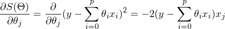
The requirement of simultaneity means that the derivative should be calculated with the old values of theta, you should not first calculate the first parameter, then the second, etc., because after changing the first parameter separately, the derivative will also change its value. Pseudo-code simultaneous change:
for i in train_samples: new_theta[1] = old_theta[1] + a * derivative(old_theta) new_theta[2] = old_theta[2] + a * derivative(old_theta) old_theta = new_theta If we calculate the values of the parameters one by one, then this will no longer be a gradient descent. Suppose we have a three-dimensional figure, and if we calculate the parameters one by one, then we can think of this process as moving only one coordinate at a time — one small step along the x coordinate, then a step along the y coordinate, and so on. steps, instead of moving in the direction of the antigradient vector.
The above variant of the algorithm is called a packet gradient descent. The number of repetitions can be replaced by the phrase "Repeat until it converges." This phrase means that the parameters will be adjusted until the previous and current values of the cost function are equal. This means that a local or global minimum has been found and the algorithm will not go on. In practice, equality cannot be achieved and the limit of convergence is introduced.
. It is established by some small value and the stopping criterion is that the difference between the previous and current values is less than the limit of convergence - this means that the minimum has been reached with the required accuracy. Higher accuracy (less ) - more iterations of the algorithm. It looks something like this: while abs(S_current - S_previous) >= Epsilon: # do something Since the post suddenly stretched out, I would like to finish it on this - in the next part I will continue to analyze the gradient descent for linear regression with OLS.
Continued .
To run the examples you need: numpy, matplotlib.
ImageMagick is required to run examples that create animations.
The materials used in the article - github.com/m9psy/neural_network_habr_guide
Source: https://habr.com/ru/post/307312/
All Articles