Pattern recognition in R using convolutional neural networks from the MXNet package
This is a detailed instruction for pattern recognition in R using the deep convolutional neural network provided by the MXNet package. This article provides a reproducible example of how to get 97.5% accuracy in a face recognition task on R.
I think some preface is still needed. I am writing this instruction based on two considerations. The first is to provide everyone with a fully reproducible example. The second is to give answers to already raised questions. Please note that this is only my way to address this problem, it is definitely not the only one, and definitely not the best.
I'm going to use both Python 3.x (for receiving and preprocessing data) and R (actually, solving the problem), so it makes sense to install both. The requirements for R packages are:
')
As for Python 3.x, install both Numpy and Scikit-learn . It may also be worthwhile to install the Anaconda distribution, which has a number of pre-installed popular packages for data analysis and machine learning .
Once you have it all worked, you can proceed.
I am going to use the Olivetti face pack . This data set is a collection of 64-by-64-pixel images, in 0-256 grayscale.
The data set contains 400 images of 40 people. With 10 instances for each person usually use uncontrolled or semi- controlled algorithms, but I am going to try and use a specific controlled method.
First you need to scale the image on a scale from 0 to 1. This is done automatically by the function that we are going to use to load the dataset, so you should not worry about it, but you need to know that it has already been done. If you are going to use your own images, pre- scale them on a scale from 0 to 1 (or -1; 1, although the first one works better with neural networks, based on my experience). Below is a Python script that needs to be executed to load a dataset. Simply change the paths to your values and execute from the IDE or terminal.
In fact, this piece of code does the following: loads the data, changes the size of the pictures by X, and saves the numpy arrays to a .csv file.
Array x is a tensor (tensor is a beautiful name for a multidimensional matrix) of size (400, 64, 64): this means that array x contains 400 copies of matrices 64 by 64 (read images). If in doubt, simply output the first elements of the tensor and try to understand the data structure, taking into account what you already know. For example, from the description of a data set, we know that we have 400 instances, each of which is an image 64 by 64 pixels. We smooth the tensor x to a matrix of 400 by 4096 in size. That is, each matrix 64 by 64 (image) is now converted (smoothed) into a horizontal vector 4096 long.
As for y, it is already a vertical vector of size 400. It does not need to be changed.
Look at the resulting .csv file and make sure all conversions are clear.
Now we will use EBImage to resize the images to 28 by 28 pixels, and generate the training and test data sets. You ask why I resize images. For some reason, my computer doesn’t like 64-by-64-pixel images, and every time I launch a model with data, an error occurs. Poorly. But it is tolerable, since we can get good results with smaller pictures (but you can, of course, try to run from 64 to 64 pixels if you do not have such a problem). So:
This part should be clear enough if you are not sure what the output looks like, you should look at the rs_df dataset . This should be a 400x785 dataset, approximately like this:
label, pixel1, pixel2, ..., pixel784
0, 0.2, 0.3, ..., 0.1
Now the most interesting, let's build a model. Below is the script that was used to train and test the model. Below are my comments and explanations to the code.
After loading the training and test dataset, I use the
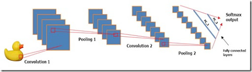
Regarding the structure of the model, this is a variation of the LeNet model using the hyperbolic tangent as an activation function instead of “Relu” (transformed linear node), 2 convolutional layers, 2 layers of a subsample, 2 fully connected layers and a standard multi-variable logistic conclusion.
Each convolutional layer uses a 5x5 core and is applied to a fixed set of filters. Watch this wonderful video to get a feel for convolutional layers. Layers of the subsample use the classic “maximize” approach.
My tests have shown that tanh works much better than sigmoid and Relu, but you can try other activation functions if you wish.
As for the hyperparameters of the model, the level of training is slightly higher than usual, but it works fine as long as the number of periods is 480. The series size, equal to 40, also works well. These hyperparameters are obtained by trial and error. It was possible to do a search on the overlapping bands, but I did not want to over-complicate the code, so I used the proven method - trial and error.
At the end you should get an accuracy of 0.975.
In general, this model was fairly easy to configure and run. When running on a CPU, training takes 4-5 minutes: a little long if you want to experiment, but still acceptable for work.
Considering the fact that we didn’t work with the data parameters at all and performed only the simplest and most common preprocessing steps, it seems to me that the results are quite good. Of course, if we wanted to achieve higher “real” accuracy, we would need to do more cross-checks (which would inevitably take a long time).
Thank you for reading, and I hope this article has helped you understand how to configure and run this particular model.
The dataset source is the Olivetti face set created by AT & T Laboratories Cambridge.
Foreword
I think some preface is still needed. I am writing this instruction based on two considerations. The first is to provide everyone with a fully reproducible example. The second is to give answers to already raised questions. Please note that this is only my way to address this problem, it is definitely not the only one, and definitely not the best.
Requirements
I'm going to use both Python 3.x (for receiving and preprocessing data) and R (actually, solving the problem), so it makes sense to install both. The requirements for R packages are:
')
- MXNet . This package will provide the model that we are going to use in this article, in fact, a deep convolutional neural network. You will not need a GPU version, the CPU will be sufficient for this task, although it may run slower. If this happens, use the GPU version.
- EBImage . This package has many tools for working with images. With him, working with images is a pleasure, the documentation is very clear and quite simple.
As for Python 3.x, install both Numpy and Scikit-learn . It may also be worthwhile to install the Anaconda distribution, which has a number of pre-installed popular packages for data analysis and machine learning .
Once you have it all worked, you can proceed.
Data set
I am going to use the Olivetti face pack . This data set is a collection of 64-by-64-pixel images, in 0-256 grayscale.
The data set contains 400 images of 40 people. With 10 instances for each person usually use uncontrolled or semi- controlled algorithms, but I am going to try and use a specific controlled method.
First you need to scale the image on a scale from 0 to 1. This is done automatically by the function that we are going to use to load the dataset, so you should not worry about it, but you need to know that it has already been done. If you are going to use your own images, pre- scale them on a scale from 0 to 1 (or -1; 1, although the first one works better with neural networks, based on my experience). Below is a Python script that needs to be executed to load a dataset. Simply change the paths to your values and execute from the IDE or terminal.
# -*- coding: utf-8 -*- # from sklearn.datasets import fetch_olivetti_faces import numpy as np # Olivetti olivetti = fetch_olivetti_faces() x = olivetti.images y = olivetti.target # print("Original x shape:", x.shape) X = x.reshape((400, 4096)) print("New x shape:", X.shape) print("y shape", y.shape) # numpy np.savetxt("C://olivetti_X.csv", X, delimiter = ",") np.savetxt("C://olivetti_y.csv", y, delimiter = ",", fmt = '%d') print("\nDownloading and reshaping done!") ################################################################################ # ################################################################################ # # Original x shape: (400, 64, 64) # New x shape: (400, 4096) # y shape (400,) # # Downloading and reshaping done! In fact, this piece of code does the following: loads the data, changes the size of the pictures by X, and saves the numpy arrays to a .csv file.
Array x is a tensor (tensor is a beautiful name for a multidimensional matrix) of size (400, 64, 64): this means that array x contains 400 copies of matrices 64 by 64 (read images). If in doubt, simply output the first elements of the tensor and try to understand the data structure, taking into account what you already know. For example, from the description of a data set, we know that we have 400 instances, each of which is an image 64 by 64 pixels. We smooth the tensor x to a matrix of 400 by 4096 in size. That is, each matrix 64 by 64 (image) is now converted (smoothed) into a horizontal vector 4096 long.
As for y, it is already a vertical vector of size 400. It does not need to be changed.
Look at the resulting .csv file and make sure all conversions are clear.
Little pre-processing in R
Now we will use EBImage to resize the images to 28 by 28 pixels, and generate the training and test data sets. You ask why I resize images. For some reason, my computer doesn’t like 64-by-64-pixel images, and every time I launch a model with data, an error occurs. Poorly. But it is tolerable, since we can get good results with smaller pictures (but you can, of course, try to run from 64 to 64 pixels if you do not have such a problem). So:
# 64 64 28 28 # rm(list=ls()) # EBImage require(EBImage) # X <- read.csv("olivetti_X.csv", header = F) labels <- read.csv("olivetti_y.csv", header = F) # rs_df <- data.frame() # : for(i in 1:nrow(X)) { # Try-catch result <- tryCatch({ # ( ) img <- as.numeric(X[i,]) # 64x64 ( EBImage) img <- Image(img, dim=c(64, 64), colormode = "Grayscale") # 28x28 img_resized <- resize(img, w = 28, h = 28) # ( , !) img_matrix <- img_resized@.Data # img_vector <- as.vector(t(img_matrix)) # label <- labels[i,] vec <- c(label, img_vector) # rs_df rbind rs_df <- rbind(rs_df, vec) # print(paste("Done",i,sep = " "))}, # ( ). ! error = function(e){print(e)}) } # . - , - . names(rs_df) <- c("label", paste("pixel", c(1:784))) # #------------------------------------------------------------------------------- # . . # set.seed(100) # df shuffled <- rs_df[sample(1:400),] # train_28 <- shuffled[1:360, ] test_28 <- shuffled[361:400, ] # write.csv(train_28, "C://train_28.csv", row.names = FALSE) write.csv(test_28, "C://test_28.csv", row.names = FALSE) # ! print("Done!") This part should be clear enough if you are not sure what the output looks like, you should look at the rs_df dataset . This should be a 400x785 dataset, approximately like this:
label, pixel1, pixel2, ..., pixel784
0, 0.2, 0.3, ..., 0.1
Model building
Now the most interesting, let's build a model. Below is the script that was used to train and test the model. Below are my comments and explanations to the code.
# rm(list=ls()) # MXNet require(mxnet) # #------------------------------------------------------------------------------- # train <- read.csv("train_28.csv") test <- read.csv("test_28.csv") # train <- data.matrix(train) train_x <- t(train[, -1]) train_y <- train[, 1] train_array <- train_x dim(train_array) <- c(28, 28, 1, ncol(train_x)) test_x <- t(test[, -1]) test_y <- test[, 1] test_array <- test_x dim(test_array) <- c(28, 28, 1, ncol(test_x)) # #------------------------------------------------------------------------------- data <- mx.symbol.Variable('data') # conv_1 <- mx.symbol.Convolution(data = data, kernel = c(5, 5), num_filter = 20) tanh_1 <- mx.symbol.Activation(data = conv_1, act_type = "tanh") pool_1 <- mx.symbol.Pooling(data = tanh_1, pool_type = "max", kernel = c(2, 2), stride = c(2, 2)) # conv_2 <- mx.symbol.Convolution(data = pool_1, kernel = c(5, 5), num_filter = 50) tanh_2 <- mx.symbol.Activation(data = conv_2, act_type = "tanh") pool_2 <- mx.symbol.Pooling(data=tanh_2, pool_type = "max", kernel = c(2, 2), stride = c(2, 2)) # flatten <- mx.symbol.Flatten(data = pool_2) fc_1 <- mx.symbol.FullyConnected(data = flatten, num_hidden = 500) tanh_3 <- mx.symbol.Activation(data = fc_1, act_type = "tanh") # fc_2 <- mx.symbol.FullyConnected(data = tanh_3, num_hidden = 40) # . , .. - . NN_model <- mx.symbol.SoftmaxOutput(data = fc_2) # #------------------------------------------------------------------------------- # mx.set.seed(100) # . CPU. devices <- mx.cpu() # #------------------------------------------------------------------------------- # model <- mx.model.FeedForward.create(NN_model, X = train_array, y = train_y, ctx = devices, num.round = 480, array.batch.size = 40, learning.rate = 0.01, momentum = 0.9, eval.metric = mx.metric.accuracy, epoch.end.callback = mx.callback.log.train.metric(100)) # #------------------------------------------------------------------------------- # predicted <- predict(model, test_array) # predicted_labels <- max.col(t(predicted)) - 1 # sum(diag(table(test[, 1], predicted_labels)))/40 ################################################################################ # ################################################################################ # # 0.975 # After loading the training and test dataset, I use the
data.matrix function to turn each dataset into a numeric matrix. Remember, the first column of data is the tags associated with each picture. Make sure you remove the tags from train_array and test_array . After separating the tags and dependent variables, you need to tell MXNet to process the data. I do this on line 19 with the following piece of code: “dim (train_array) <- c (28, 28, 1, ncol (train_x))” for the training set and on line 24 for the test set. Thus, we actually tell the model that the training data consists of ncol (train_x) samples (360 pictures) of size 28x28. The number 1 indicates that the pictures are in grayscale, i.e., that they have only 1 channel. If the pictures were in RGB, 1 would have to be replaced by 3, just as many channels would have pictures.Regarding the structure of the model, this is a variation of the LeNet model using the hyperbolic tangent as an activation function instead of “Relu” (transformed linear node), 2 convolutional layers, 2 layers of a subsample, 2 fully connected layers and a standard multi-variable logistic conclusion.
Each convolutional layer uses a 5x5 core and is applied to a fixed set of filters. Watch this wonderful video to get a feel for convolutional layers. Layers of the subsample use the classic “maximize” approach.
My tests have shown that tanh works much better than sigmoid and Relu, but you can try other activation functions if you wish.
As for the hyperparameters of the model, the level of training is slightly higher than usual, but it works fine as long as the number of periods is 480. The series size, equal to 40, also works well. These hyperparameters are obtained by trial and error. It was possible to do a search on the overlapping bands, but I did not want to over-complicate the code, so I used the proven method - trial and error.
At the end you should get an accuracy of 0.975.
Conclusion
In general, this model was fairly easy to configure and run. When running on a CPU, training takes 4-5 minutes: a little long if you want to experiment, but still acceptable for work.
Considering the fact that we didn’t work with the data parameters at all and performed only the simplest and most common preprocessing steps, it seems to me that the results are quite good. Of course, if we wanted to achieve higher “real” accuracy, we would need to do more cross-checks (which would inevitably take a long time).
Thank you for reading, and I hope this article has helped you understand how to configure and run this particular model.
The dataset source is the Olivetti face set created by AT & T Laboratories Cambridge.
Source: https://habr.com/ru/post/307242/
All Articles