Solving the problem of binary classification in the XGboost machine learning package

This article will discuss the problem of binary classification of objects and its implementation in one of the most productive machine learning packages "R" - "XGboost" (Extreme Gradient Boosting).
In real life, we often encounter a class of problems where the object of prediction is a nominative variable with two gradations, when we need to predict the outcome of a certain event or make decisions in binary expression based on the data model. For example, if we assess the situation on the market and our goal is to make an unequivocal decision whether it makes sense to invest in a specific instrument at a given time, whether the buyer will buy the product under investigation or not, whether the borrower will pay the loan or leave the employee in the near future etc.

In the general case, binary classification is used to predict the probability of occurrence of a certain event by the values ​​of a set of features. To do this, we introduce the so-called dependent variable (outcome of the event), which takes only one of two values ​​(0 or 1) and a set of independent variables (also called characteristics, predictors, or regressors).

At once I will make a reservation that in "R" there are several linear functions for solving similar problems, such as "glm" from the standard package of functions, but here we consider a more advanced version of the binary classification implemented in the "XGboost" package. This model, the multiple winner of Kaggle competitions, is based on building binary decision trees capable of supporting multi-stream data processing. About the features of the implementation of the family of models "Gradient Boosting" you can read here:

http://www.ncbi.nlm.nih.gov/pmc/articles/PMC3885826/
https://en.wikipedia.org/wiki/Gradient_boosting

Let's take a test data set (Train) and build a model to predict the survival of passengers during a crash:

data(agaricus.train, package='xgboost') data(agaricus.test, package='xgboost') train <- agaricus.train test <- agaricus.test 

If, after a transformation, the matrix contains many zeros, then such an array of data must first be converted into a sparse matrix - in this form, the data will take up much less space, and accordingly the processing time will be much shorter. Here the Matrix library will help us today the latest available version 1.2-6 contains a set of functions for converting to dgCMatrix on a column basis.
In the case when the already compacted matrix (sparse matrix) after all transformations does not fit in the RAM, in such cases use the special program “Vowpal Wabbit”. This is an external program that can handle datasets of any size, reading from many files or databases. “Vowpal Wabbit” is an optimized parallel machine learning platform developed for distributed computing by “Yahoo!” You can read about it in some detail at these links:

https://habrahabr.ru/company/mlclass/blog/248779/
https://en.wikipedia.org/wiki/Vowpal_Wabbit

The use of sparse matrices allows us to construct a model using text variables with their preliminary transformation.
So, to build the predictor matrix, first load the necessary libraries:

  library(xgboost) library(Matrix) library(DiagrammeR) 

When converting to the matrix, all categorical variables will be transposed, respectively, the function with the standard booster will include their values ​​in the model. The first thing to do is to remove variables with unique values ​​from the data set, such as “Passenger ID”, “Name” and “Ticket Number”. We carry out the same actions with a test dataset, which will be used to calculate predicted outcomes. For clarity, I downloaded data from local files that I downloaded in the corresponding dataset Kaggle. For the model, it will need the following table columns:

  input.train <- train[, c(3,5,6,7,8,10,11,12)] input.test <- test[, c(2,4,5,6,7,9,10,11)]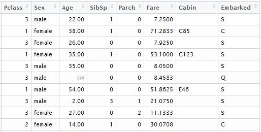 

separately form a vector of known outcomes for learning the model

  train.lable <- train$Survived 

Now it is necessary to perform data conversion so that statistically significant variables are taken into account when training the model into accounting. Perform the following conversions:
Replace variables containing categorical data with numeric values. It should be borne in mind that ordered categories, such as 'good', 'normal', 'bad' can be replaced by 0,1,2. Non-ordered data with relatively low selectivity, such as 'gender' or 'Country Name', can be left unchanged as factors; after being converted into a matrix, they are transposed into the appropriate number of columns with zeros and ones. For numeric variables, all unassigned and missing values ​​must be processed. There are at least three options: you can replace them with 1, 0, or a more acceptable option would be to replace them with an average value in the column of this variable.
When using the “XGboost” package with a standard booster (gbtree), variable scaling can be avoided, unlike other linear methods such as “glm” or “xgboost” with a linear booster (gblinear).

Basic package information can be found at the following links:

https://github.com/dmlc/xgboost
https://cran.r-project.org/web/packages/xgboost/xgboost.pdf

Returning to our code, as a result we got a table of the following format:

next, replace all missing entries with the arithmetic average value of the predictor column

  if (class(inp.column) %in% c('numeric', 'integer')) { inp.table[is.na(inp.column), i] <- mean(inp.column, na.rm=TRUE) 

after preprocessing, we do the conversion to "dgCMatrix":

  sparse.model.matrix(~., inp.table) 

It makes sense to create a separate function for preprocessing predictors and converting to sparse.model.matrix format, for example, the variant with the "for" cycle is given below. To optimize performance, you can vectorize an expression using the "apply" function.

  spr.matrix.conversion <- function(inp.table) { for (i in 1:ncol(inp.table)) { inp.column <- inp.table [ ,i] if (class(inp.column) == 'character') { inp.table [is.na(inp.column), i] <- 'NA' inp.table [, i] <- as.factor(inp.table [, i]) } else if (class(inp.column) %in% c('numeric', 'integer')) { inp.table [is.na(inp.column), i] <- mean(inp.column, na.rm=TRUE) } } return(sparse.model.matrix(~.,inp.table)) } 

Then we use our function and convert the actual and test tables into sparse matrices:

  sparse.train <- preprocess(train) sparse.test <- preprocess(test) 

To build a model, we need two data sets: the data matrix that we have just created and the vector of actual outcomes with a binary value (0.1).
The "xgboost" function is the most convenient to use. The “XGBoost” implements a standard booster based on binary decision trees.
To use “XGboost”, we must choose one of three parameters: general parameters, booster parameters and destination parameters:
• General parameters - we define which booster will be used, linear or standard.
The remaining parameters of the booster depend on which booster we chose in the first step:
• Parameters of learning tasks - we determine the purpose and scenario of learning
• Command line parameters - used to determine the command line mode when using “xgboost.”.

General view of the “xgboost” function that we use:

  xgboost(data = NULL, label = NULL, missing = NULL, params = list(), nrounds, verbose = 1, print.every.n = 1L, early.stop.round = NULL, maximize = NULL, ...) 

"data" - the data matrix format ("matrix", "dgCMatrix", local data file or "xgb.DMatrix".)
"label" is the vector of the dependent variable. If this field was a component of the original parameter table, then it should be excluded before processing and converting it to a matrix, in order to avoid the transitivity of the links.
"nrounds" is the number of constructed decision trees in the final model.
"objective" - ​​through this parameter we transfer the tasks and assignments of training the model. For logistic regression, there are 2 options:
"reg: logistic" is a logistic regression with a continuous value from 0 to 1;
"binary: logistic" is a logistic regression with a binary prediction value. For this parameter, you can set a specific threshold for the transition from 0 to 1. By default, this value is 0.5.
Details on the model parameterization can be found at this link.

http: //xgboost/parameter.md% 20at% 20master% 2020% 20dmlc / xgboost% 20% 5GitHub
Now we are starting to create and train the “XGBoost” model:

  set.seed(1) xgb.model <- xgboost(data=sparse.train, label=train$Survived, nrounds=100, objective='reg:logistic') 

if desired, you can extract the tree structure using the function xgb.model.dt.tree (model = xgb). Next, use the standard function “predict” to form a predictive vector:

  prediction <- predict(xgb.model, sparse.test) 

and finally, save the data in a readable format

  solution <- data.frame(prediction = round(prediction, digits = 0), test) write.csv(solution, 'solution.csv', row.names=FALSE, quote=FALSE) 

adding a vector of predicted outcomes, we get the following table:

Now we’ll go back and briefly look at the model we just created. To display the decision trees, you can use the functions "xgb.model.dt.tree" and "xgb.plot.tree". So, the last function will give us a list of selected trees with a model fit factor:

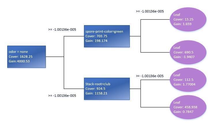
Using the xgb.plot.tree function, we will also see a graphical representation of trees, although it should be noted that in the current version, it is far from the best way implemented in this function and is of little use. Therefore, for clarity, I had to manually reproduce an elementary decision tree based on the standard Train data model.

Testing the statistical significance of variables in the model will tell us how to optimize the matrix of predictors for learning the XGB model. It is best to use the xgb.plot.importance function in which we pass an aggregated parameter importance table.

  importance_frame <- xgb.importance(sparse.train@Dimnames[[2]], model = xgb) xgb.plot.importance(importance_frame) 

So, we have considered one of the possible implementations of logistic regression based on the “xgboost” function package with a standard booster. At the moment, I recommend using the “XGboost” package as the most advanced group of machine learning models. Currently, predictive models based on the logic of “XGboost” are widely used in financial and market forecasting, marketing, and many other areas of applied analytics and machine intelligence.