Mathematics for artificial neural networks for beginners, part 1 - linear regression
Table of contents
Part 1 - linear regression
Part 2 - Gradient Descent
Part 3 - Gradient Descent continued
Introduction
With this post I will start the cycle “Neural networks for beginners”. It is dedicated to artificial neural networks (suddenly). The purpose of the cycle is to explain this mathematical model. Often, after reading such articles, I still had a feeling of understatement, misunderstandings - the National Assembly was still a “black box” - it is generally known how they are structured, what they do, what they know and what the input and output data are known for. But nevertheless a complete, comprehensive understanding is missing. And modern libraries with very pleasant and convenient abstractions only reinforce the feeling of the “black box”. I can not say that this is definitely bad, but it’s also never too late to understand the tools used. Therefore, my primary goal is to provide a detailed explanation of the structure of neural networks so that absolutely no one has any questions about their structure; so that the NA does not seem like magic. Since this is not a mathematical treatise, I will confine myself to describing several methods in simple language (but not excluding formulas, of course), providing explanatory illustrations and examples.
The cycle is designed for the basic university level of mathematical reading. The code will be written in Python3.5 with numpy 1.11. The list of other auxiliary libraries will be at the end of each post. Absolutely everything will be written from scratch. The MNIST base is chosen as the test subject. These are black and white, centered images of handwritten numerals of 28 * 28 pixels. By default, 60,000 images are marked for training, and 10,000 for testing. In the examples, I will not change the default distribution.
Sample images from MNIST:
')

I will not focus on the structure of MNIST and just lay out the code that loads the database and saves it in the right format. This format will be used in the following examples:
loader.py
import struct import numpy as np import requests import gzip import pickle TRAIN_IMAGES_URL = "http://yann.lecun.com/exdb/mnist/train-images-idx3-ubyte.gz" TRAIN_LABELS_URL = "http://yann.lecun.com/exdb/mnist/train-labels-idx1-ubyte.gz" TEST_IMAGES_URL = "http://yann.lecun.com/exdb/mnist/t10k-images-idx3-ubyte.gz" TEST_LABELS_URL = "http://yann.lecun.com/exdb/mnist/t10k-labels-idx1-ubyte.gz" def downloader(url: str): response = requests.get(url, stream=True) if response.status_code != 200: print("Response for", url, "is", response.status_code) exit(1) print("Downloaded", int(response.headers.get('content-length', 0)), "bytes") decompressed = gzip.decompress(response.raw.read()) return decompressed def load_data(images_url: str, labels_url: str) -> (np.array, np.array): images_decompressed = downloader(images_url) # Big endian 4 unsigned int, 4 magic, size, rows, cols = struct.unpack(">IIII", images_decompressed[:16]) if magic != 2051: print("Wrong magic for", images_url, "Probably file corrupted") exit(2) image_data = np.array(np.frombuffer(images_decompressed[16:], dtype=np.dtype((np.ubyte, (rows * cols,)))) / 255, dtype=np.float32) labels_decompressed = downloader(labels_url) # Big endian 2 unsigned int, 4 magic, size = struct.unpack(">II", labels_decompressed[:8]) if magic != 2049: print("Wrong magic for", labels_url, "Probably file corrupted") exit(2) labels = np.frombuffer(labels_decompressed[8:], dtype=np.ubyte) return image_data, labels with open("test_images.pkl", "w+b") as output: pickle.dump(load_data(TEST_IMAGES_URL, TEST_LABELS_URL), output) with open("train_images.pkl", "w+b") as output: pickle.dump(load_data(TRAIN_IMAGES_URL, TRAIN_LABELS_URL), output) Linear regression
Linear regression is a method for restoring dependency between two variables. Linear means that we assume that variables are expressed through an equation of the form:
 Epsilon here is a model error. Also, for clarity and simplicity, we will deal with a one-dimensional model - multidimensionality does not add complexity, but the illustration will not work. For a moment, we’ll forget about MNIST and generate some data stretched into a line. We also rewrite the regression model (hypothesis) as follows:
  . y with a cap is the predicted value of the model.
  1 and 2 - unknown parameters - the main task is to find these parameters, and x is a free variable, its values are known to us. We formulate the problem again and in a slightly different language - we have a set of experimental data in the form of pairs of values
  and you need to find a straight line on which these values are located, to find a line that would best summarize the experimental data. Some code to generate data:
generate_linear.py
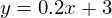
import numpy as np import matplotlib.pyplot as plt TOTAL = 200 STEP = 0.25 def func(x): return 0.2 * x + 3 def generate_sample(total=TOTAL): x = 0 while x < total * STEP: yield func(x) + np.random.uniform(-1, 1) * np.random.uniform(2, 8) x += STEP X = np.arange(0, TOTAL * STEP, STEP) Y = np.array([y for y in generate_sample(TOTAL)]) Y_real = np.array([func(x) for x in X]) plt.plot(X, Y, 'bo') plt.plot(X, Y_real, 'g', linewidth=2.0) plt.show() As a result, something like this should turn out - quite accidentally for an unprepared human eye:
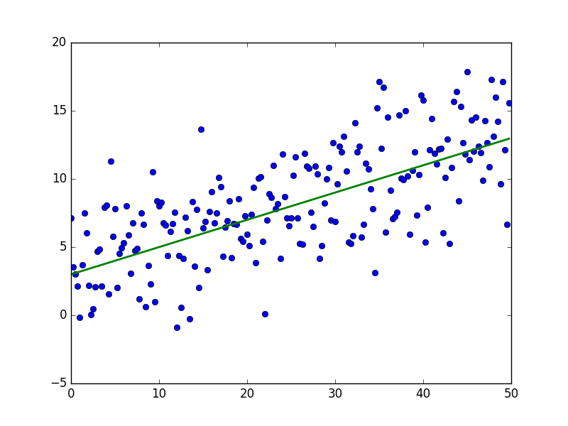
The green line is “base” - data is randomly distributed above and below this line, the distribution is uniform. The equation for the green line is:
Least square method
The essence of MNCs is to find such parameters.
 so that the predicted value is closest to real. Graphically, it expresses something like this:
Code
import matplotlib.pyplot as plt plt.plot([1, 2, 3, 4, 5], [4, 2, 9, 9, 5], 'bo') plt.plot([1, 2, 3, 4, 5], [3, 5, 7, 9, 11], '-ro') plt.show() 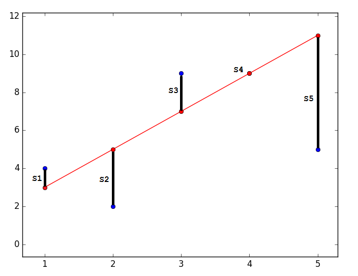
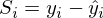
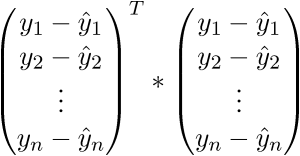
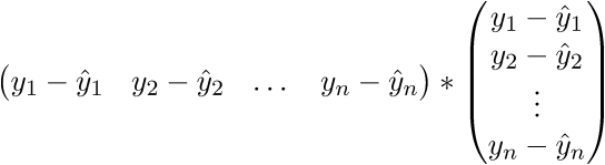
The closest - means that the vector
 should have the shortest possible length. Since the vector is not the only one, it is postulated that the sum of the squares of the lengths of all vectors should tend to the minimum, taking into account the vector of parameters . In my opinion, quite logical method, speculative. Nevertheless, there is a mathematical proof of the correctness of this Remarque method: by length we mean the Euclidean metric , although this is not necessary. Remark 2 : note that the sum of the squares. Again, no one forbids trying to minimize just the sum of the lengths . In this picture, the red dots are the predicted value (
  ), blue - obtained as a result of the experiment (y without a cap).
  - this is just the difference between them, the length of the vector.
Mathematically, it looks like this:
 - it is required to find such a vector
  in which the expression
  reaches a minimum. The function f in this expression is:
 or
or
I had been thinking for a long time whether it was worth going straight to the vectorization of the code and as a result the article would be too long without it. Therefore, we introduce new notation:
 - vector consisting of the values of the dependent variable y -
  - vector of parameters -
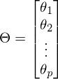
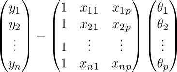
A is the matrix of the values of the free variable x. In this case, the first column is 1 (x_0 is missing) -
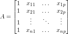 . In the one-dimensional case in matrix A there are only two columns -
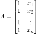
After the new notation, the equation of the line goes to the matrix equation of the following form:
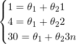
 . In this equation, 2 unknowns are predicted values and parameters. We can try to find out the parameters from the same equation, but with known values:
  Otherwise, it can be represented as a system of equations:
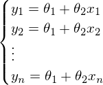
It would seem that everything is known - both the vector Y and the vector X - it remains only to solve the equation. The big problem is that the system may not have solutions - otherwise, the matrix A may not have an inverse matrix. A simple example of a system without a solution — any three \ four \ n points not on the same straight line \ plane \ hyperplane — this causes the matrix A to become non-square, which means by definition there is no inverse matrix
 .
.A vivid example of the impossibility of solving the “simple way” (using some Gauss method to solve a system):

The system looks like this:
 - It is unlikely to find solutions for such a system.
As a result, it is impossible to build a line through these three points - one can only construct an approximately correct solution.
Such a digression is an explanation of why the MNC and its brothers were needed at all. Minimizing the cost function (loss function) and the impossibility (unnecessary, harmful) of finding an absolutely exact solution are one of the most basic ideas that underlie neural networks. But they are still far away, but for now let us return to the method of least squares.
OLS tells us that it is necessary to find the minimum of the sum of squares of the vectors of the form:
 The sum of squares, taking into account that everything is transformed into a vector \ matrix can be written as follows:
 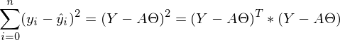 .
.I will not turn the language to call it a trivial transformation, it can be quite difficult for beginners to get away from simple variables to vectors, so I will write out all this expression completely in “open” vectors. Again, so that not a single line is misunderstood by "magic."
To begin with, simply “uncover” the vectors in accordance with their definition:
 .
.Check the dimension - for the matrix A it is equal to (n; p), and for the vector
- (p; 1), and for vector - (n; 1). As a result, we obtain the difference of two vectors of dimension (n; 1) -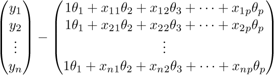
Checking the definition - by definition it turns out that each row of the right matrix is equal to
 . We write further:
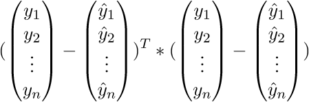


As a result, the last line is the sum of squares of length, as we need. Each time, of course, such tricks in the mind turn for a long time, but you can get used to the vector notation quickly. This has a plus for the programmer - it is more convenient to work and port the code for the GPU, where the vector traveled through the vector. I somehow ported the Perlin noise generation to the GPU and a rough understanding of the vector notation made the work quite well. There is also a minus - you have to constantly climb on the Internet to recall the identities and rules of linear algebra. After proving the fidelity of the vector notation, we proceed to further transformations:


Here the properties of matrix transposition are used - namely, the transposition of the sum and product. And also the fact that expressions
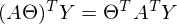 and
and  there is a constant. You can prove it by taking the dimension of the matrices from their definition and calculating the dimension of the expression after all multiplications:
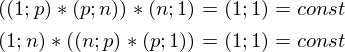
The constant can be represented as a symmetric matrix, therefore:

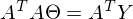
After the transformations and disclosure of brackets, it is time to solve the posed problem — to find the minimum of this expression, given
 . The minimum is quite casual - equating the first differential over to zero. In an amicable way, you must first prove that this minimum exists at all, I propose to omit the proof and spy it in the literature yourself . Intuitively, it is clear that the quadratic function is a parabola, and it has a minimum.
So,
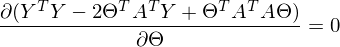


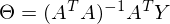
Part
 called a pseudo-inverse matrix.
Now available all the necessary formulas. The sequence of actions is as follows:
1) Generate a set of experimental data.
2) Create a matrix A.
3) Find the pseudo-inverse matrix
 .
.4) Find
After this, the problem will be solved - we will have at our disposal the parameters of a straight line that best summarizes the experimental data. Otherwise, we will have the parameters for the direct, best expressing the linear dependence of one variable on another - this is exactly what was required.
generate_linear.py
import numpy as np import matplotlib.pyplot as plt TOTAL = 200 STEP = 0.25 def func(x): return 0.2 * x + 3 def prediction(theta): return theta[0] + theta[1] * x def generate_sample(total=TOTAL): x = 0 while x < total * STEP: yield func(x) + np.random.uniform(-1, 1) * np.random.uniform(2, 8) x += STEP X = np.arange(0, TOTAL * STEP, STEP) Y = np.array([y for y in generate_sample(TOTAL)]) Y_real = np.array([func(x) for x in X]) A = np.empty((TOTAL, 2)) A[:, 0] = 1 A[:, 1] = X theta = np.linalg.pinv(A).dot(Y) print(theta) Y_prediction = A.dot(theta) error = np.abs(Y_real - Y_prediction) print("Error sum:", sum(error)) plt.plot(X, Y, 'bo') plt.plot(X, Y_real, 'g', linewidth=2.0) plt.plot(X, Y_prediction, 'r', linewidth=2.0) plt.show() And the results:
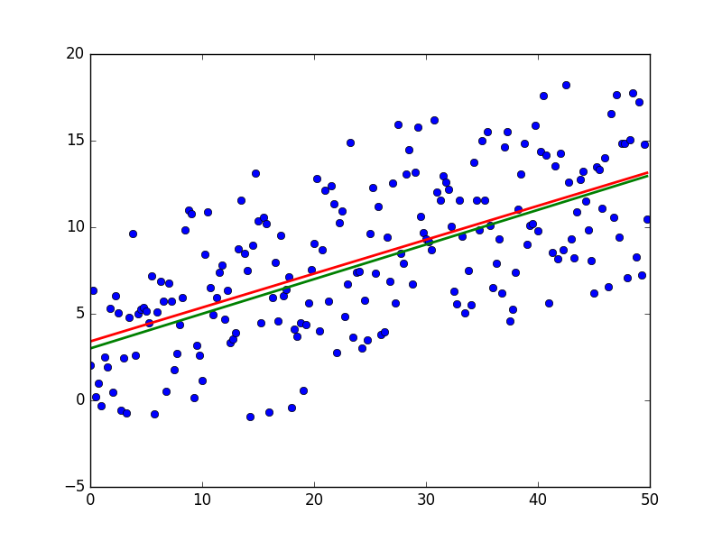
The red line was predicted and almost coincides with the green “base”. The parameters in my launch are equal: [3.40470411, 0.19575733]. Try to predict the values will not work, because while the distribution of model errors is unknown. All that can be done is to check if OLS is true for a given case, the OLS will be the appropriate and best method for generalization. Three conditions :
1) Mat expectation of errors is zero.
2) Error variance - a constant value.
3) There is no correlation of errors in different dimensions. The covariance is zero.
To do this, I added an example by calculating the required values and carried out measurements twice:
generate_linear.py
import numpy as np import matplotlib.pyplot as plt TOTAL = 200 STEP = 0.25 def func(x): return 0.2 * x + 3 def prediction(theta): return theta[0] + theta[1] * x def generate_sample(total=TOTAL): x = 0 while x < total * STEP: yield func(x) + np.random.uniform(-1, 1) * np.random.uniform(2, 8) x += STEP X = np.arange(0, TOTAL * STEP, STEP) Y = np.array([y for y in generate_sample(TOTAL)]) Y_real = np.array([func(x) for x in X]) A = np.empty((TOTAL, 2)) A[:, 0] = 1 A[:, 1] = X theta = np.linalg.pinv(A).dot(Y) print(theta) Y_prediction = A.dot(theta) error = Y - Y_prediction error_squared = error ** 2 M = sum(error) / len(error) M_squared = M ** 2 D = sum([sq - M_squared for sq in error_squared]) / len(error) print("M:", M) print("D:", D) plt.plot(X, Y, 'bo') plt.plot(X, Y_real, 'g', linewidth=2.0) plt.plot(X, Y_prediction, 'r', linewidth=2.0) plt.show() 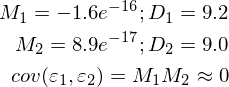
Imperfect, but without deception, everything works as expected.
The next part.
A complete list of libraries to run examples: numpy, matplotlib, requests.
The materials used in the article - https://github.com/m9psy/neural_nework_habr_guide
Source: https://habr.com/ru/post/307004/
All Articles