Stylization of images using neural networks: no mysticism, just matan
Greetings to you, Habr! Surely, you have noticed that the theme of the stylization of photographs for various artistic styles is actively discussed on these web sites of yours. Reading all these popular articles, you might think that magic is going on under the hood of these applications, and the neural network really fantasizes and redraws the image from scratch. It just so happened that our team was faced with a similar task: as part of the intra-corporate hackathon, we made video styling , because application for photos already. In this post, we'll figure out how this network "redraws" images, and analyze the articles that made this possible. I recommend to get acquainted with the previous post before reading this material and in general with the basics of convolutional neural networks . You will find a few formulas, a bit of code (I will give examples on Theano and Lasagne ), as well as a lot of pictures. This post is built in the chronological order of the articles and, accordingly, the ideas themselves. Sometimes I will dilute it with our recent experience. Here you have a boy from hell to attract attention.
Visualizing and Understanding Convolutional Networks (28 Nov 2013)
The first thing worth mentioning is an article in which the authors were able to show that the neural network is not a black box, but a completely interpretable thing (by the way, today it can be said not only about convolutional networks for computer vision). The authors decided to learn to interpret the activation of neurons of hidden layers, for this they used the deconvolutionary neural network (deconvnet) proposed several years earlier (by the way, by the same Zeiler and Fergus, who are the authors of this publication). A deconvolutional network is actually the same network with convolutions and pooling, but applied in the reverse order. In the original work on deconvnet, the network was used in unsupervised learning mode for generating images. This time, the authors applied it simply for a backward pass from the signs obtained after a direct pass through the network to the original image. The result is an image that can be interpreted as a signal that caused this activation on neurons. Naturally, the question arises: how to make a reverse pass through convolution and nonlinearity? And even more so through max-pooling, this is certainly not an invertible operation. Consider all three components.
Reverse ReLu
In convolution networks, as the activation function, ReLu (x) = max (0, x) is often used, which makes all activations on the layer not negative. Accordingly, when going back through nonlinearity, non-negative results must also be obtained. For this, the authors propose to use the same ReLu. From the point of view of the Theano architecture, it is necessary to redefine the gradient function of the operation (the infinitely valuable laptop is in the lasagna recipes , from there you will get the details of what is behind the ModifiedBackprop class).
class ZeilerBackprop(ModifiedBackprop): def grad(self, inputs, out_grads): (inp,) = inputs (grd,) = out_grads #return (grd * (grd > 0).astype(inp.dtype),) # explicitly rectify return (self.nonlinearity(grd),) # use the given nonlinearity Reverse convolution
It is a bit more complicated here, but everything is logical: it is enough to apply the transposed version of the same convolution kernel, but to the outputs from the reverse ReLu instead of the previous layer used in the forward pass. But I'm afraid that in words it is not so obvious, let's look at the visualization of this procedure ( here you will find even more visualizations of bundles).
| Convolution with stride = 1 | Back version |
|---|---|
 |  |
| Convolution with stride = 2 | Back version |
|---|---|
 |  |
Reverse pooling
This operation (unlike the previous ones) is generally not invertible. But we would still like to go through a maximum in some way back. To do this, the authors propose to use the map of where was the maximum with a direct pass (max location switches). During the backward pass, the input signal is converted into an ampling in order to approximately preserve the structure of the original signal, it’s really easier to see than to describe.

Result
The visualization algorithm is extremely simple:
- Make a straight pass.
- Select the layer of interest.
- To fix the activation of one or more neurons and reset the rest.
- Make a reverse conclusion.
Each gray square in the image below corresponds to the visualization of the filter (which is used for convolution) or the weights of one neuron, and each color image is the part of the original image that activates the corresponding neuron. For clarity, neurons within a single layer are grouped into subject groups. In general, it suddenly turned out that the neural network learns exactly what Hubel and Wazel wrote about in the work on the structure of the visual system , for which they were awarded the Nobel Prize in 1981. Thanks to this article, we got a visual representation of what a convolutional neural network learns on each layer. It is this knowledge that will allow later to manipulate the contents of the generated image, but this is still far away, the next few years were spent on improving the methods of "trepanning" neural networks. In addition, the authors of the article proposed a method for analyzing how best to build the convolutional neural network architecture to achieve the best results (although they did not win ImageNet 2013, but they got to the top; UPD : it turns out they won, Clarifai is what they are).
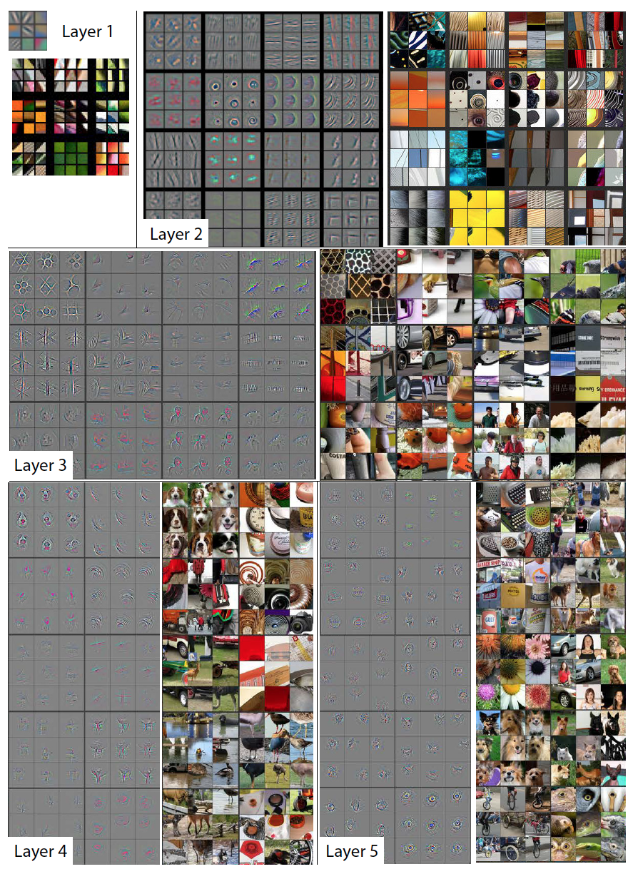
Here is an example of visualization of activations using deconvnet, today this result looks already so-so, but then it was a breakthrough.
Deep Inside Convolutional Networks: Visualizing Image Classification Models and Saliency Maps (19 Apr 2014)
This article is devoted to the study of the methods of knowledge visualization, enclosed in a convolutional neural network. The authors propose two visualization methods based on gradient descent.
Class Model Visualization
So, imagine that we have a trained neural network to solve the problem of classification into a certain number of classes. Denote by  activation value of the output neuron, which corresponds to class c . Then the following optimization problem gives us exactly the image that maximizes the selected class:
This task is easy to solve using Theano. Usually we ask the framework to take a derivative with respect to the model parameters, but this time we assume that the parameters are fixed and the derivative is taken from the input image. The following function selects the maximum value of the output layer and returns a function that calculates the derivative of the input image.
def compile_saliency_function(net): """ Compiles a function to compute the saliency maps and predicted classes for a given minibatch of input images. """ inp = net['input'].input_var outp = lasagne.layers.get_output(net['fc8'], deterministic=True) max_outp = T.max(outp, axis=1) saliency = theano.grad(max_outp.sum(), wrt=inp) max_class = T.argmax(outp, axis=1) return theano.function([inp], [saliency, max_class]) You must have seen strange images on the Internet with dog faces - DeepDream. In the original article, the authors use the following process to generate images that maximize the selected class:
- Initialize the initial image with zeros.
- Calculate the derivative value of this image.
- Change the image by adding to it the resulting image from the derivative.
- Return to step 2 or exit the loop.
These are the following images:
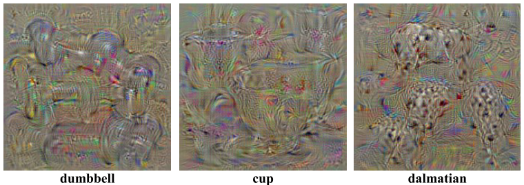
And if you initialize the first image of a real photo and run the same process? But at each iteration we will choose a random class, reset the others and calculate the value of the derivative, then we will get such a deep dream.
Why are there so many dog faces and eyes? It's simple: there are almost 200 dogs in 1000 imad from 1000 classes, they have eyes. And also many classes where people are just there.
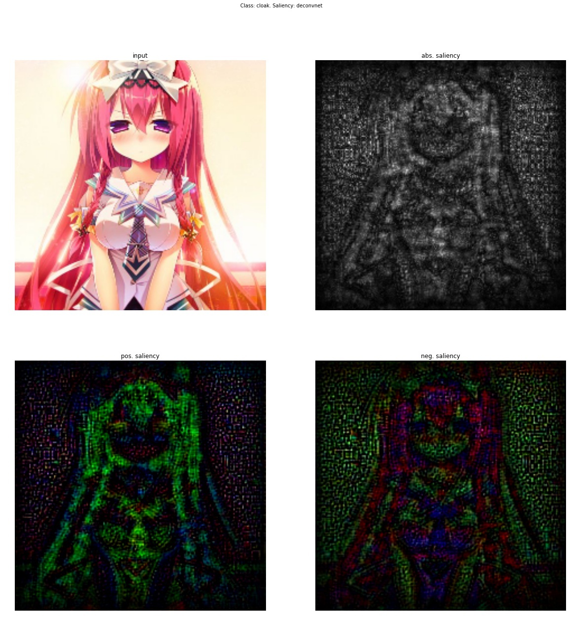
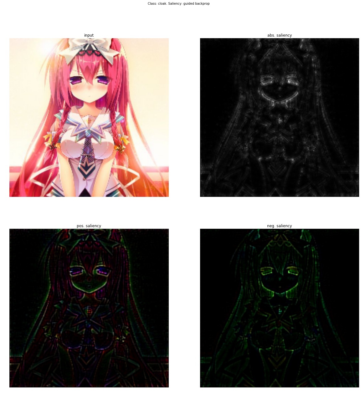
Class Saliency Extraction
If we initialize this process with a real photo, stop after the first iteration and draw the value of the derivative, we will get such an image, adding it to the original one, we will increase the activation value of the selected class.

Again the result is "so-so." It is important to note that this is a new way of visualizing activations (nothing prevents us from fixing the values of activations not on the last layer, but generally on any layer of the network and taking a derivative of the input image). The following article will combine both of the previous approaches and give us a tool for how to set up a transfer style that will be described later.
Striving for Simplicity: The All Convolutional Net (13 Apr 2015)
This article is generally not about visualization, but about the fact that replacing a pooling with a convolution with a large straid does not lead to a loss of quality. But as a by-product of their research, the authors proposed a new way of visualizing the features, which they used to more accurately analyze what the model was learning. Their idea is as follows: if we simply take a derivative, then with deconvolution, those features that were less than zero in the input image do not go back (using ReLu for the input image). And this leads to the fact that negative values appear on the propped back image. On the other hand, if you use deconvnet, then another ReLu is taken from the ReLu derivative - this allows you not to skip back negative values, but as you have seen the result is “so-so”. But what if you combine these two methods?
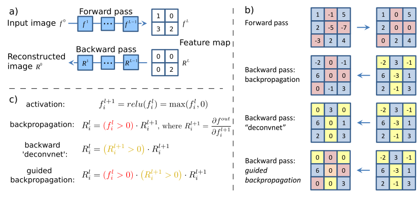
class GuidedBackprop(ModifiedBackprop): def grad(self, inputs, out_grads): (inp,) = inputs (grd,) = out_grads dtype = inp.dtype return (grd * (inp > 0).astype(dtype) * (grd > 0).astype(dtype),) Then get a completely clean and interpretable image.
Go deeper
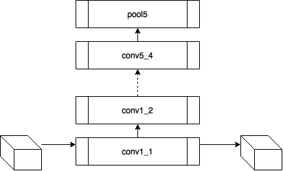
Now let's think, what does this give us? Let me remind you that each convolutional layer is a function that receives a three-dimensional tensor as an input and also produces a three-dimensional tensor as an output, perhaps another dimension d x w x h ; d epth is the number of neurons in the layer, each of them generates a plate (feature map) of size w igth x h eight.
Let's try the following experiment on the VGG-19 network:
- for each layer of the neural network, we will sort the plates by the value of the sum of activations inside the plates
 - this will give us the most pronounced features on the image (in one plate there are activations of the same feature in different spatial coordinates);
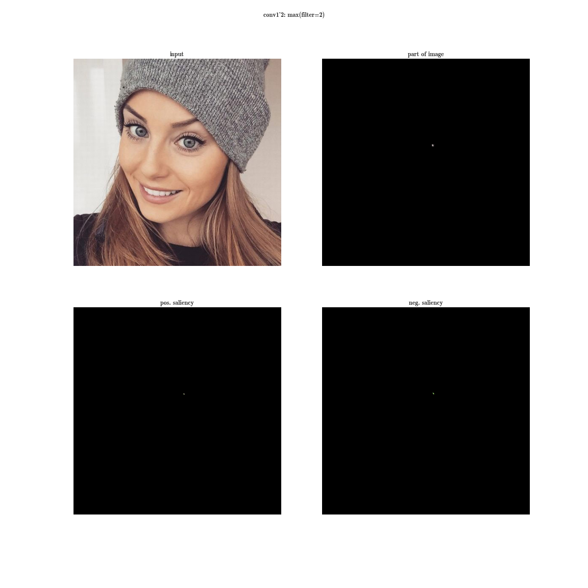
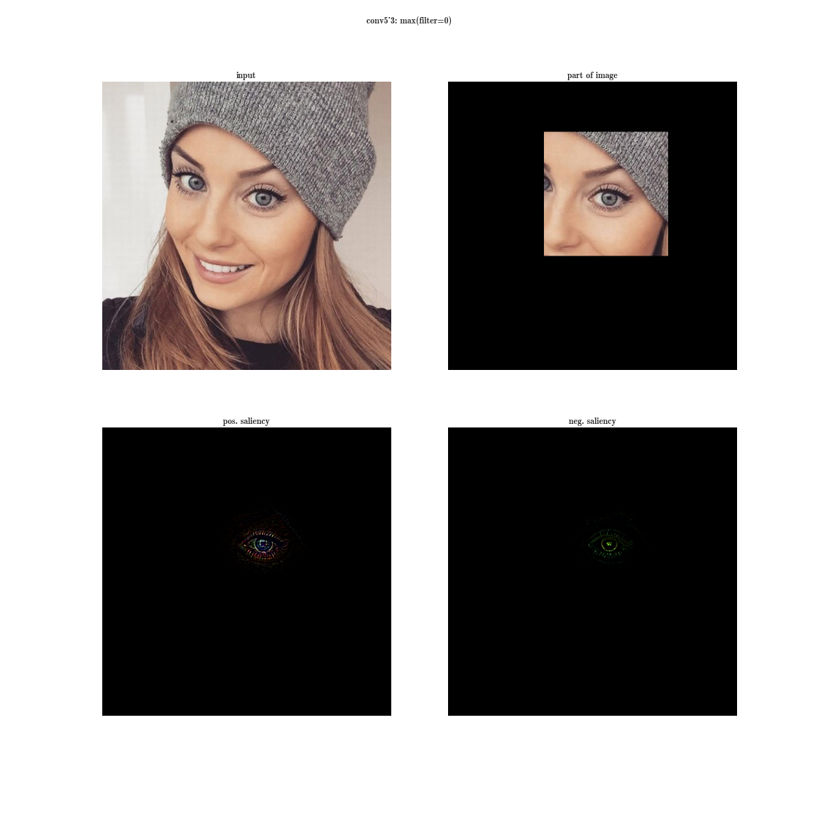
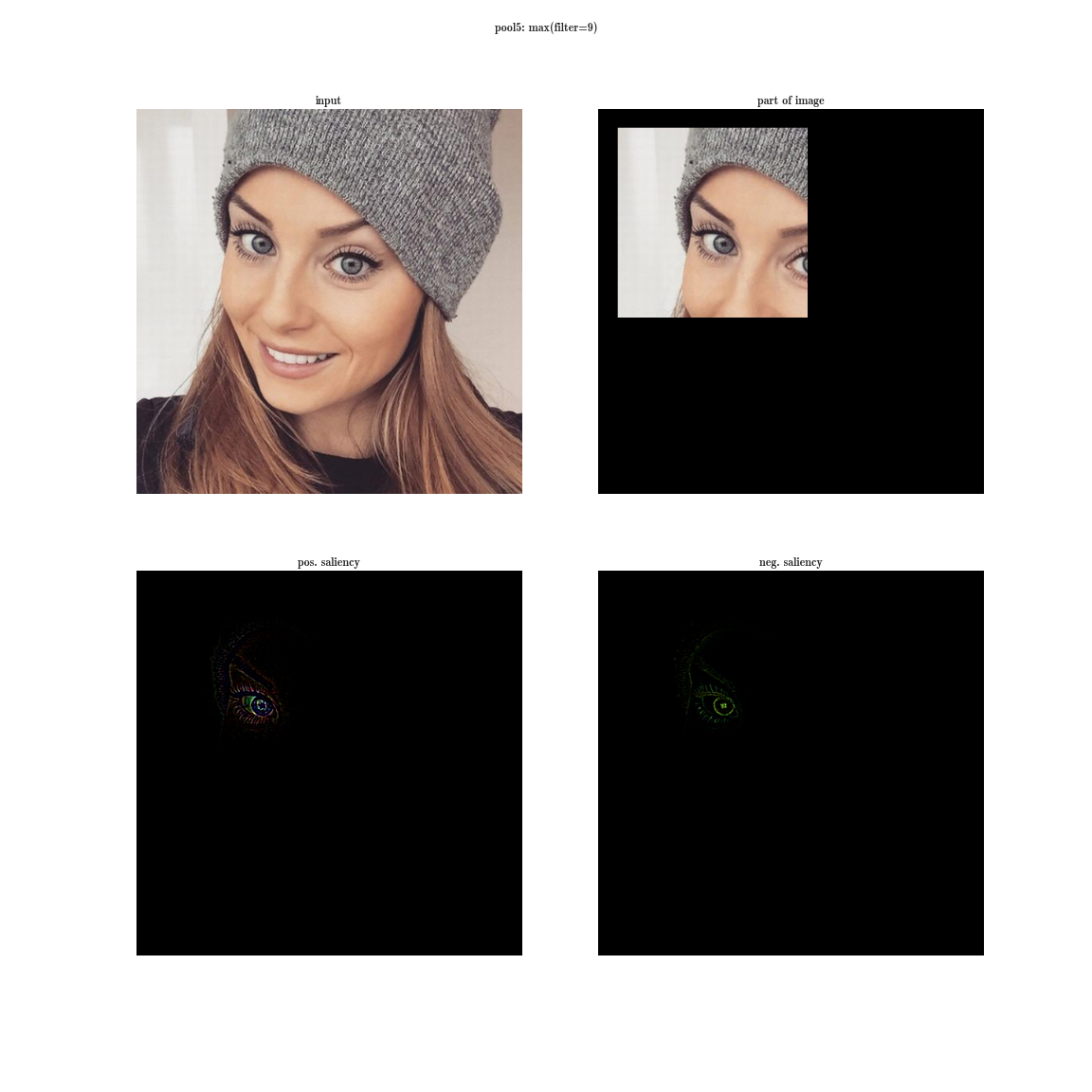
 - then on each plate we will choose the maximum element - this will give us the position where this feature is most clearly expressed;
- And now we take the derivative of the input image for a fixed value of one position on one plate and zeroed other values in the layer - this will give us an idea of the feature, as well as the receptive area of this neuron (what area of the image this neuron is looking at).
Yes, you see almost nothing, because the receptive region is very small, it is the second convolution of 3x3, respectively, the general area of 5x5. But having increased, we will see that the feature is just a gradient detector.
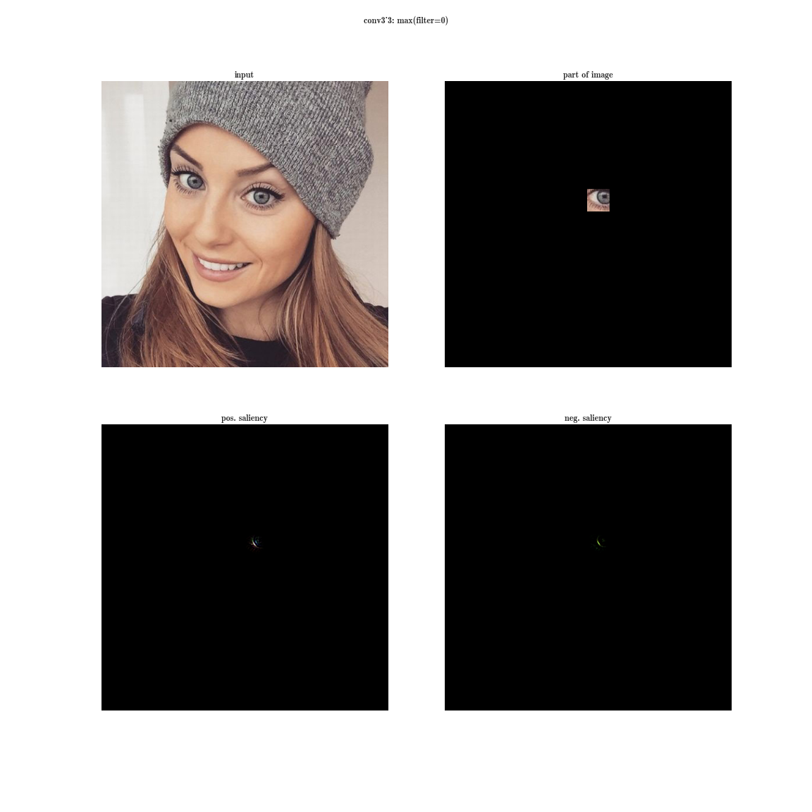
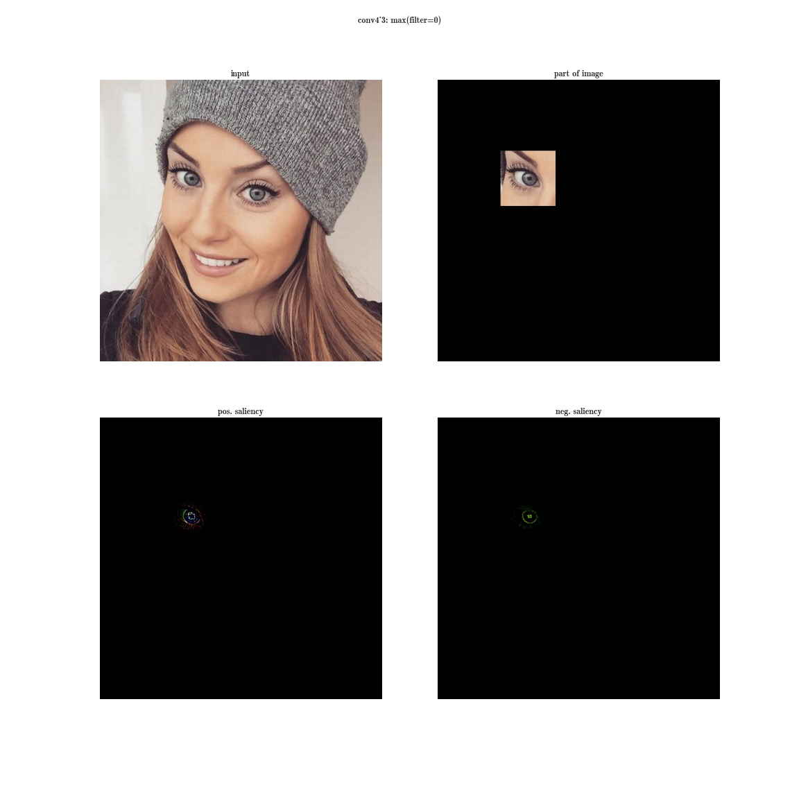
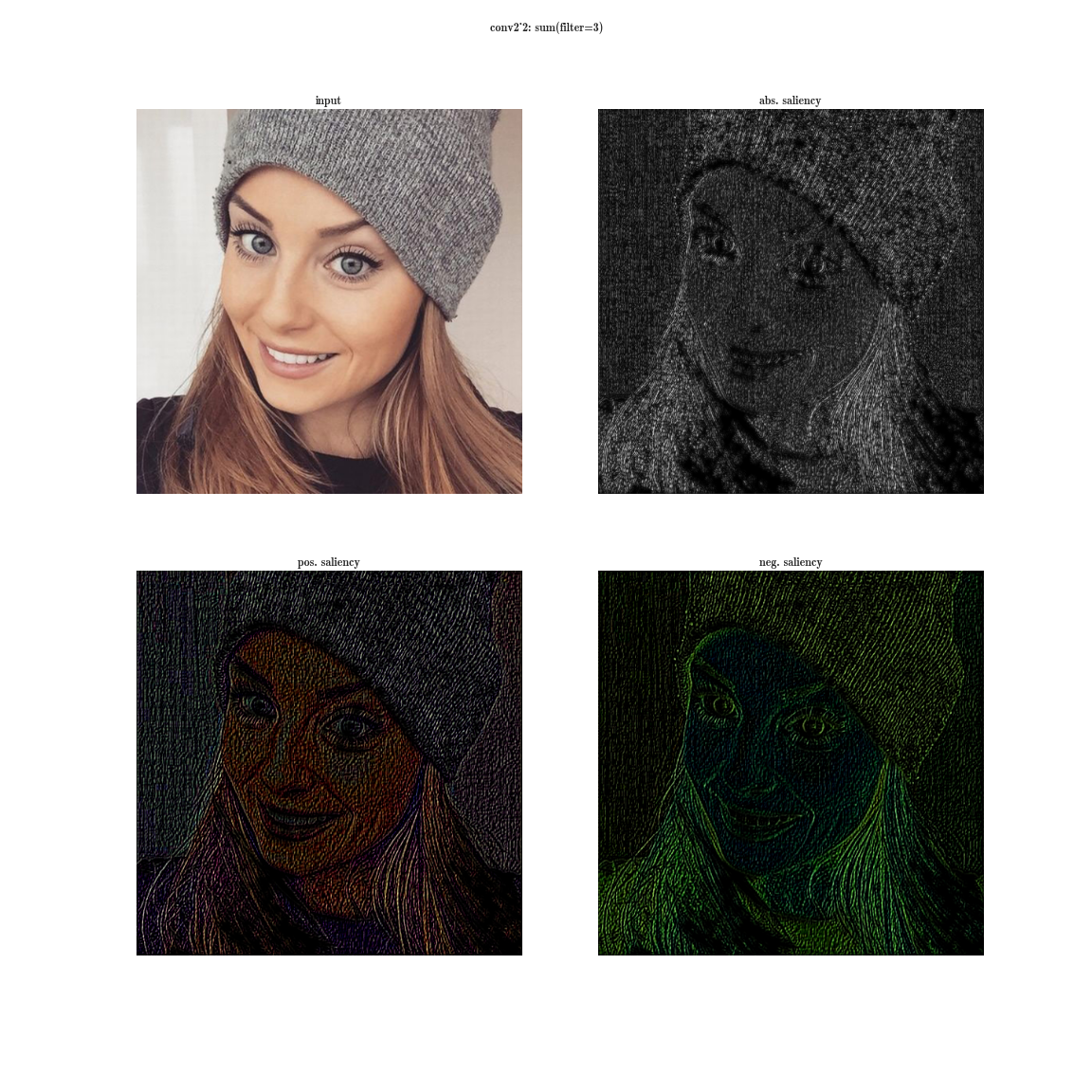
Now imagine that instead of a maximum on a plate, we will take the derived value of the sum of all the elements of the plate on the input image. Then obviously the receptive region of the neuron group will cover the entire input image. For the early layers, we will see bright maps, from which we conclude that these are color detectors, then gradients, then borders, and so on, in the direction of complicating patterns. The deeper the layer, the duller the image is. This is explained by the fact that the deeper layers have a more complex pattern, which they detect, and a complex pattern appears less frequently than a simple one, and therefore the activation map dims. The first method is suitable for understanding layers with complex patterns, and the second one is for simple ones.


You can download a more complete database of activations for several images here and here .
A Neural Algorithm of Artistic Style (2 Sep 2015)
So, a couple of years have passed since the first successful trepanning of the neural network. We (in the sense of humanity) have a powerful tool in their hands, which allows us to understand what the neural network is learning, and also to remove what we don’t really want what it would learn. The authors of this article are developing a method that allows one image to generate a similar card of activations for some target image, and perhaps even more than one - this is the basis of stylization. At the entrance we give white noise, and with a similar iterative process as in deep dream we bring this image to one whose feature maps are similar to the target image.
Content loss
As already mentioned, each layer of the neural network produces a three-dimensional tensor of a certain dimension.
Denote the output of the i-th layer from the input as  . Then if we minimize the weighted sum of the residuals between the input image
  and by some image, to which we aspire c , we get exactly what we need. Probably.
For experiments with this article, you can use this magic laptop , there are calculations (both on the GPU and on the CPU). The GPU is used to calculate the neural network features and the value of the cost function. Theano returns a function that can calculate the gradient of the objective function eval_grad from the input image x . This is then fed into lbfgs and an iterative process is started.
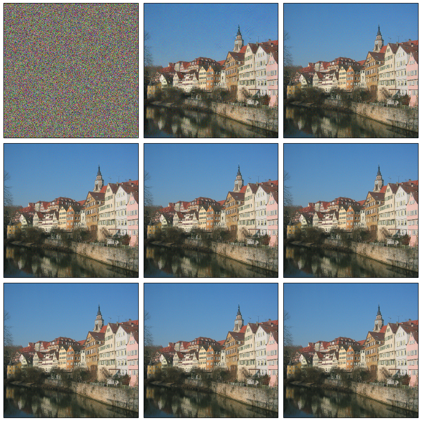
# Initialize with a noise image generated_image.set_value(floatX(np.random.uniform(-128, 128, (1, 3, IMAGE_W, IMAGE_W)))) x0 = generated_image.get_value().astype('float64') xs = [] xs.append(x0) # Optimize, saving the result periodically for i in range(8): print(i) scipy.optimize.fmin_l_bfgs_b(eval_loss, x0.flatten(), fprime=eval_grad, maxfun=40) x0 = generated_image.get_value().astype('float64') xs.append(x0) If we launch the optimization of such a function, we will quickly get an image similar to the target one. Now we are able to recreate from white noise images similar to some content-image.
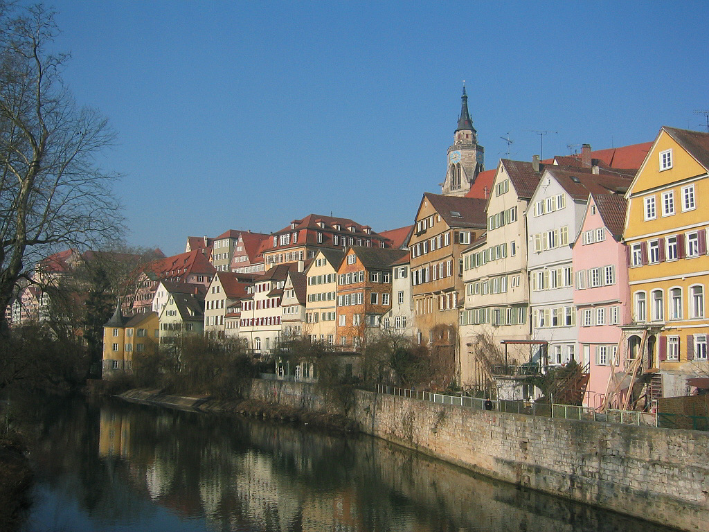
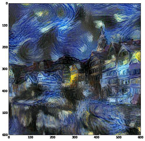
Content Image
Optimization process
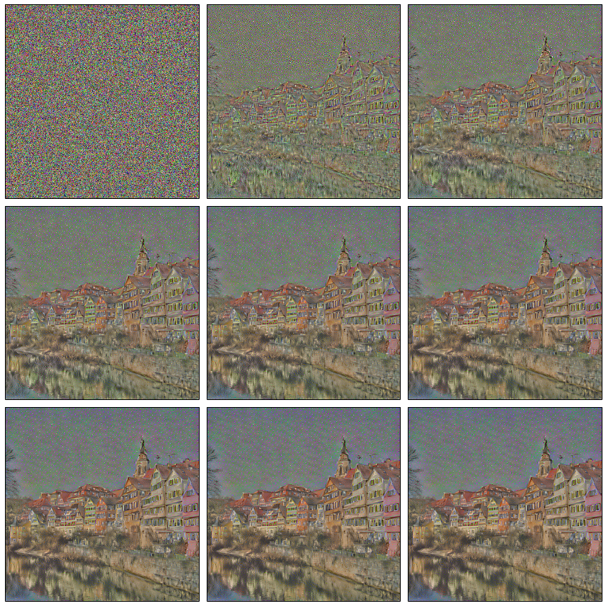
It is easy to notice two features of the resulting image:
- lost colors - this is the result of the fact that in the concrete example only the conv4_2 layer was used (or, in other words, the weight w was non-zero for it, and zero for the other layers); as you remember, it is the early layers that contain information about colors and gradient transitions, and the later ones contain information about larger details, which we observe — colors are lost, but no content;
- some of the houses “went”, i.e. straight lines are slightly curved - this is because the deeper layer, the less information about the spatial position of the feature it contains (the result of convolutions and pooling).
Adding early layers immediately corrects the situation with colors.
I hope by this point you have felt that you can control what will be redrawn onto the image from the white noise.
Style loss
And so we got to the most interesting: how can we convey the style? What is style? Obviously, the style is not something that we optimized in Content Loss, because there is a lot of information about the spatial positions of features. So the first thing to do is in some way remove this information from the views received at each layer.
The author suggests the following method. Take the tensor at the exit of a certain layer, turn on the spatial coordinates and calculate the covariance matrix between the dies. We denote this transformation as G. What did we actually do? We can say that we calculated how often the signs inside the plate are found in pairs, or, in other words, we approximated the distribution of signs in the plates with a multidimensional normal distribution.

Then Style Loss is entered as follows, where s is an image with a style:
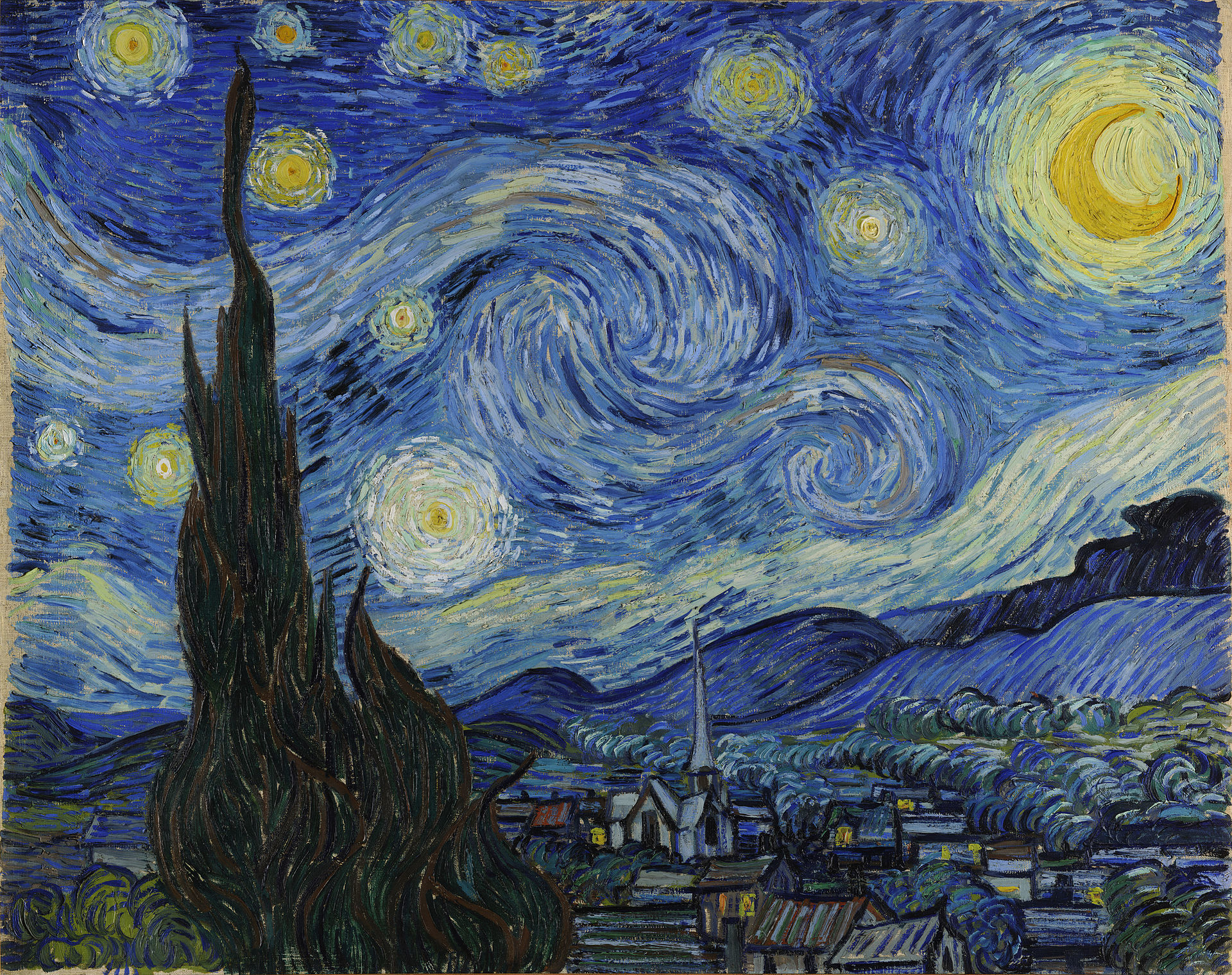
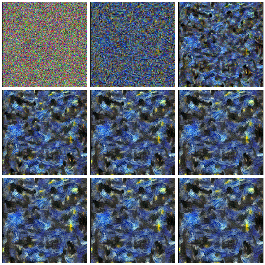
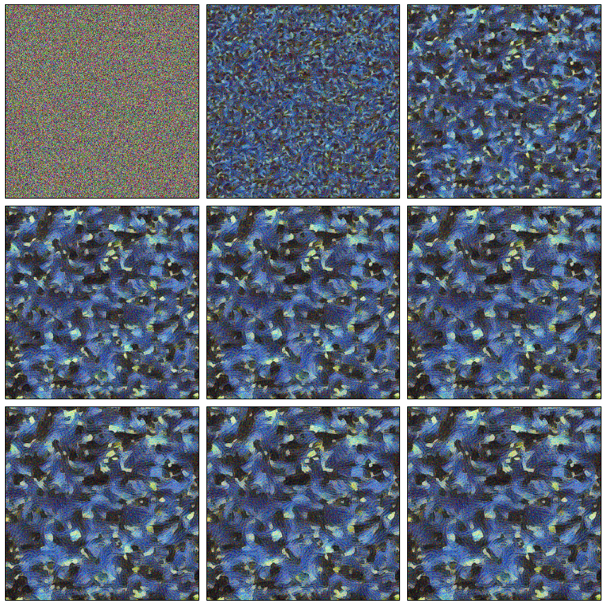
Let's try for Vincent? In principle, we will get something expected - the noise in the Van Gogh style, the information about the spatial arrangement of features is completely lost.
And what if instead of a style image to put a photo? It will turn out already familiar features, familiar colors, but the spatial position is completely lost.
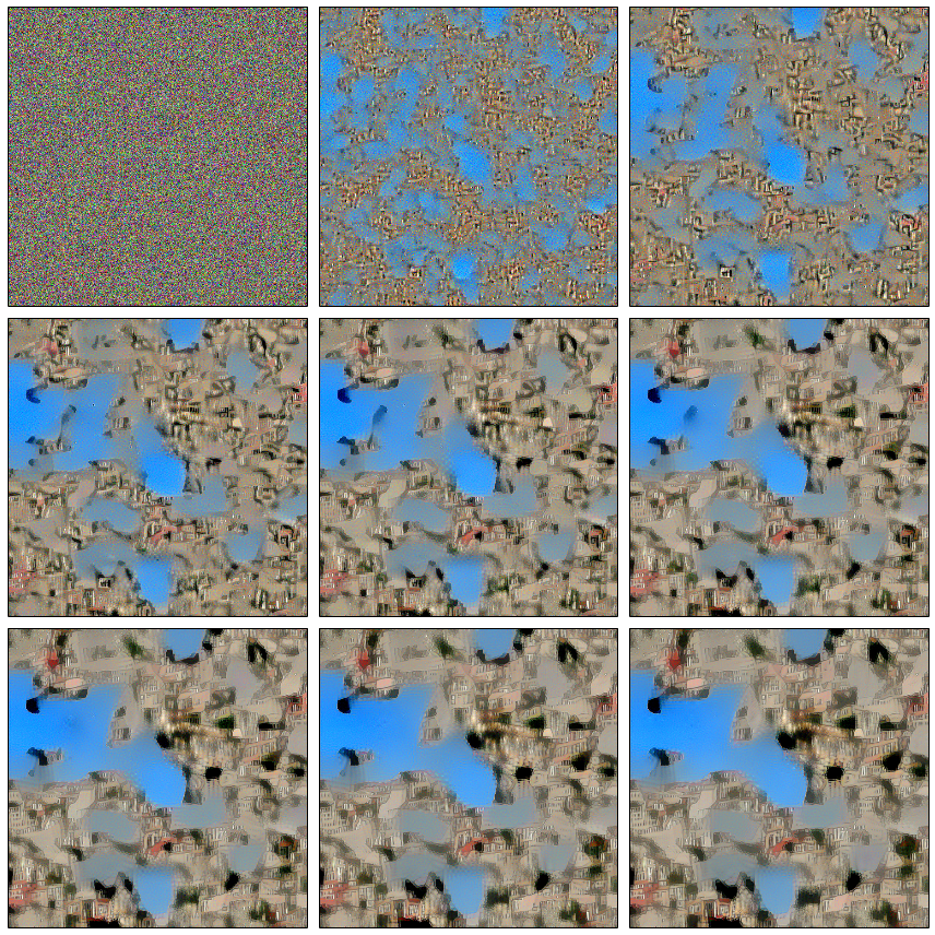
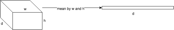
Surely you wondered about why we calculate the covariance matrix, and not something else? After all, there are many ways to aggregate features so that spatial coordinates are lost. This is really an open question, and if you take something very simple, the result will not change dramatically. Let's check this, we will not calculate the covariance matrix, but simply the average value of each plate.
Combined Loss
Naturally, there is a desire to mix these two functions of value. Then we will generate such an image from white noise that it will save the signs from the content-image (which have a binding to spatial coordinates), as well as the “style” signs that are not tied to spatial coordinates, i.e. we will hope that the details of the image content will remain intact from their places, but will be redrawn with the right style.

In fact, there is also a regularizer, but we omit it for simplicity. It remains to answer the following question: which layers (weights) should be used for optimization? And I am afraid that I have no answer to this question, and the authors of the article, too. They have a suggestion to use the following, but this does not mean at all that another combination will work worse, too much search space. The only rule that follows from the understanding of the model: it makes no sense to take the next layers, because their signs will not differ much from each other, therefore a layer from each group of conv * _1 is added to the style.
# Define loss function losses = [] # content loss losses.append(0.001 * content_loss(photo_features, gen_features, 'conv4_2')) # style loss losses.append(0.2e6 * style_loss(art_features, gen_features, 'conv1_1')) losses.append(0.2e6 * style_loss(art_features, gen_features, 'conv2_1')) losses.append(0.2e6 * style_loss(art_features, gen_features, 'conv3_1')) losses.append(0.2e6 * style_loss(art_features, gen_features, 'conv4_1')) losses.append(0.2e6 * style_loss(art_features, gen_features, 'conv5_1')) # total variation penalty losses.append(0.1e-7 * total_variation_loss(generated_image)) total_loss = sum(losses) The final model can be represented as follows.

Attempt to control the process
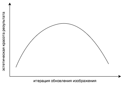
Let's remember the previous parts, already two years before the current article, other scientists investigated what the neural network really learns. Armed with all these articles, you can create visualizations of features of various styles, different images, different resolutions and sizes, and try to figure out which layers to take with what weight. But even re-weighting the layers does not give full control over what is happening. The problem here is more conceptual: we are optimizing the wrong function ! How so, you ask? The answer is simple: this function minimizes the discrepancy ... well, you understand. But what we really want is that we like the image. The convex combination of content and style loss functions is not a measure of what our mind considers beautiful. It was noted that if you continue styling for too long, the cost function naturally falls lower and lower, but the aesthetic beauty of the result drops sharply.
Well, okay, there is another problem. Suppose we found a layer that retrieves the features we need. Suppose some texture triangular. But this layer still contains many other features, such as circles, which we really do not want to see in the resulting image. Generally speaking, if one could hire a million Chinese, one could visualize all the features of the style image, and just look at all that we need, and only include them in the cost function. But for obvious reasons, it is not so simple. But what if we just remove all the circles that we don’t want to see on the result from the style image? Then the activation of the corresponding neurons that react to the circles will simply not work. And, of course, this will not appear in the resulting image. The same with flowers. Imagine a bright image with lots of color. The distribution of colors will be very blurred over the entire space, the distribution of the resulting image will be the same, but in the process of optimization those peaks that were on the original will surely be lost. It turned out that a simple decrease in the color depth of the color palette solves this problem. The distribution density of most colors will be near zero, and there will be large peaks in several areas. Thus, by manipulating the original in Photoshop, we manipulate the features that are extracted from the image. It is easier for a person to express his desires visually, rather than trying to formulate them in the language of mathematics. Until. As a result, designers and managers, armed with photoshop and scripts for visualizing signs, achieved three times faster results better than the one that mathematicians did with programmers.
| Original | Degraded version |
|---|---|
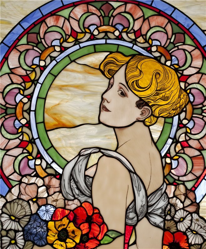 | 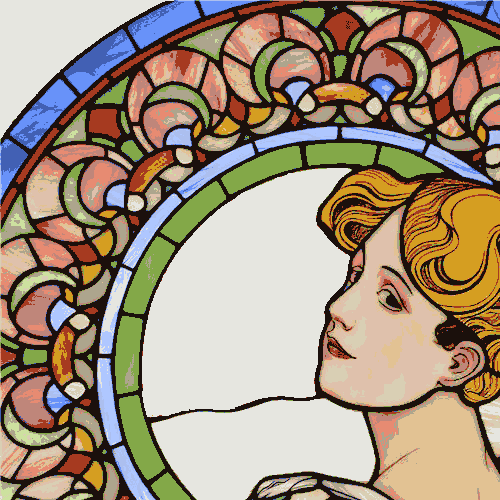 |
Style
results
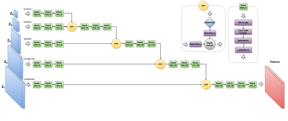
Texture Networks: Feed-Forward Synthesis of Textures and Stylized Images (Mar 10, 2016)
, . . , lbfgs , . , , 10-15 . . . 17 , . , , ( Style Loss ). , , , .
, . -. , z , . - , .. Loss- , .
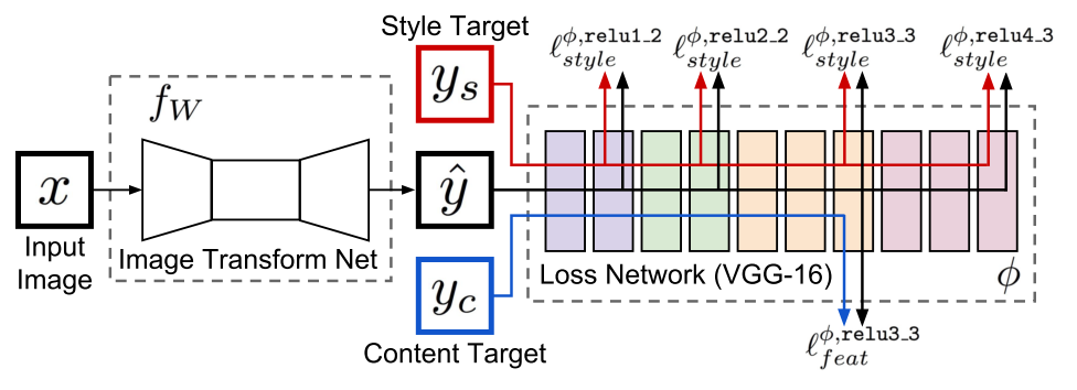
Perceptual Losses for Real-Time Style Transfer and Super-Resolution (27 Mar 2016)
, , 17 , . residual learning .
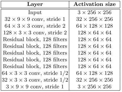
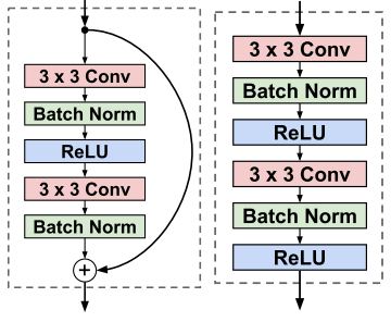
residual block conv block.
, ( ).
Ending
:
- :
:
- Theano
- Lasagne
- Lasagne/Recipes , + — ; , TF, - 8 , 700
- Lasagne/Recipes/examples/Saliency Maps and Guided Backpropagation
- Lasagne/Recipes/examples/styletransfer/Art Style Transfer
- Torch
- resnet-like Chainer
- Gatys' Torch, resnet-like ; lbfgs
')
Source: https://habr.com/ru/post/306916/
All Articles