Representation of movements in 3D modeling: interpolation, approximation, and Lie algebra
In this article I would like to talk about one interesting mathematical technique that, being very interesting and useful, is little known to a wide circle of people involved in computer graphics.
How many different ways are there to represent an ordinary rotation in three-dimensional space? Most people who have ever done 3D graphics or 3D modeling will immediately name three main common options:
People with rich experience will add here for some reason not popular fourth paragraph:
I would like to talk about the fifth way of representing rotations, which is sympathetic because it is convenient for parametrization, allows you to effectively build polynomial approximations of these parametrization, carry out spherical interpolation, and most importantly, is universal - with minimal changes it works for all kinds of movements. If you have ever needed a method that would allow you to easily make “an analogue of slerp, but not for pure rotations, but for voluntary movements, and even scaling”, then read this article.
')
I will start with a mathematical description of where the fifth way of representing rotations arises, what exactly is the emerging parametrization, but everyone can skip this section and go straight to the practical part at the end of the article .
Rotations of an object in three-dimensional space (and, in general, any movement of an object) from a mathematical point of view are a typical example of a structure called “group” . The group operation here is “combining” when one motion is first applied and then the second; This combination is obviously also a movement. The unit of the group is the "change nothing" trivial movement. For any movement, you can find the reverse movement, allowing "to return everything as it was." On the practical side, in relation to geometry, the existence of a group often speaks of the existence of some kind of “feature” of a given movement, which is preserved within the group. For example, if we moved an object somewhere by pure rotation, then we can also return it back by pure rotation . The group of motions of the Euclidean space preserves the distance between the points of the object being moved. The symmetry group of a cube consists of 48 movements that translate a cube into itself. This is something that everyone knows more or less.
It is easy, however, to note that the group of rotations is arranged in a certain sense “more interesting” than the group of symmetries of the cube. So, we know that for rotations it is possible to interpolate continuous motion between any two points (to find a function that smoothly and continuously rotates an object from one position to another), whereas for the 48 elements of the symmetry group of the cube this is obviously impossible. Another interesting property is the ability to locally parameterize the elements of this group by triples of numbers (for example, Euler angles). In mathematical terms, all these properties are formalized with the phrase “a group of rotations is a smooth manifold” . That is, we can imagine the space of all possible rotations in three-dimensional space as a certain multidimensional surface like a sphere. Only here the usual sphere is a two-dimensional surface and it can be placed ( nested ) in three-dimensional space, and the space of rotations is a three-dimensional hypersurface and in order to depict it you will need four-dimensional space; and to do this without self-intersections, a six-dimensional one, and the surface for a group of rotations obtained in this space would resemble a bagel rather than a sphere topologically. But the mathematics there is almost the same, so I will use the usual two-dimensional sphere to intuitively illustrate the concept of “smooth manifold”.
We now consider the continuous motion of an object, given by the function of the object's position depending on the moment of time f (t). For example, f (0) can determine the initial position of the object, f (1) - the final, and f (0.5) will then correspond to the position of the object on the “middle of the road” from the starting point to the final one. Since the individual positions of the object are points on our smooth manifold, then considering f (t) at different points, we can build on our “sphere” a chain of points connecting the starting and ending points on the “sphere”; in the limit, as it is easy to understand, this chain unites into a continuous curve. That is, different curves on our manifold are different trajectories of the movement of objects and vice versa.

Fig. 1. The group of rotations as a smooth manifold (sphere): the points correspond to the initial and final positions of the object, the curve passing through the sphere - the trajectory of its movement
Recall now that we still have not some abstract variety, but a group; and this group has two operations: “multiplication” and “taking the inverse element”. We can "act" with these operations on the "sphere." For example, we can make a so-called. “Left shift by the element g”, multiplying all the points on the sphere to the left by g , i.e. replacing each element a with g * a . Since we have a group, this movement preserves our “sphere” as a whole, but it moves certain marked points inside it. Intuitive interpretation: since we have a group of turns, we can turn our sphere on any of these turns.

Fig. 2. The action of the group on itself as a turn of the sphere
If such operations of the group on itself (multiplication and inversion) do not spoil the smoothness of the curves previously defined on it (they are smooth mappings of the sphere onto themselves), then such a group is called a Lie group . All practically significant groups of movements are precisely Lie groups.
The next interesting observation that we can make is that for smooth curves on smooth manifolds, we can define the concept of the velocity along a curve — a tangent vector . That is, in our case of a moving object, you can determine the speed of rotation of the body at any time, and this speed will be a vector quantity . In differential geometry, there is a theorem stating that the space of all possible tangent vectors to curves at a given point of an n-dimensional manifold is the n-dimensional linear space — the tangent plane at a given point of the manifold . For example, the speed of rotation of the body can be determined by the axis of rotation and the angular velocity of rotation. If we multiply the unit vector of the axis direction by the scalar of angular velocity, then we obtain the angular velocity vector , the direction of which defines the axis, and the length - the speed of rotation. This vector will be an element of this tangent space to the group of rotations. In the illustration, I use a two-dimensional sphere as a model, therefore the tangent space there is obtained by a two-dimensional tangent plane to this sphere.

Fig. 3. The speed of rotation as a tangent vector to the trajectory of the object and the tangent plane - as the space of all possible velocities of rotation of the object at the selected point
However, due to the fact that the tangent plane is defined for a specific point of the manifold, so far we have defined the “object rotation speed” for only one specific point (a particular object position), and we would like it for any possible position. This is where the “smooth action of a manifold on itself” characteristic of Lie groups comes to the rescue: by defining the tangent vector and the tangent plane of just one point of the manifold (as a rule, one), we can further move the resulting vector and plane to any other point of variety. To do this, however, we will have to fix some specific way in which we will do this in order to avoid ambiguities, and the classical approach is to use the already mentioned left shift , i.e. use the multiplication on the left of g to calculate the tangent vector and the tangent plane at g . This is easy to give an obvious interpretation: suppose we have defined what “left rotation at a speed of 5 degrees per second” is for an object in position A. How to determine “rotation of an object to the left at a speed of 5 degrees per second” in a different position B? To do this, you just need to first give the object a turn in the old position, and then (multiply on the left) place the object in the right place with the same turn, which would lead a stationary object from position A to B. Such a notation naturally implies that the movements are from right to left : the action a * b corresponds to the action b , followed by the action a . Thus, having determined the rotation speed at one point, it is possible to further define the concept of “rotation speed” for all points in space. The resulting vector field (the mathematician will add: a left-invariant vector field ) on a Lie group is naturally associated with “just” rotational speed, without specifying exactly which point.

Fig. 4. The “rotation speed” determined at one point is naturally defined for all points of the rotation group.
As I wrote earlier, the space of all possible angular velocities at one point is a three-dimensional tangent space. Since this construction works for any tangent vectors, the words “at the point” can be removed here too; that is, it turns out simply “the space of possible angular velocities of the object”, and this space is the usual linear space of all conceivable three-dimensional vectors. This space is called a Lie algebra corresponding to a given Lie group. Why algebra? And because for this space the addition and multiplication by a scalar (space linearly ) is already naturally defined, and it is always possible to introduce a special “multiplication operation” - a Lie bracket with the following properties:
For our simple case, in addition, from points 1 and 2, the point also follows:
As applied to our case of a group of rotations, the Lie algebra, as we have already understood, is the usual three-dimensional space of vectors, and the “multiplication” in it is a well-known vector product .
Groups and Lie algebras play a prominent role in mathematics, since Lie algebra (linear space) is usually a much simpler object than the original group. For example, in our model example, the original Lie group was a tricky three-dimensional donut embedded in a six-dimensional space, and the Lie algebra was already a usual three-dimensional space. For the original elements of a Lie group, only the operation of combining rotations was defined and it was not commutative, whereas elements of a Lie algebra can be added together and multiplied by scalars. But at the same time, the Lie algebra uniquely determines the corresponding Lie group and allows determining its properties (for example, determining the type of group) through the properties of the Lie algebra, which, by and large, reduce to the dimension of the linear space and the matrix describing the Lie bracket through its action on the basis vectors . However, for practical purposes, we need another important property.
Consider an arbitrary smooth trajectory of motion f (t) in our Lie group. As already mentioned, it can be differentiated by determining the speed in each of the points of the trajectory. We now take an arbitrary element x from a Lie algebra (an arbitrary angular velocity for our model example). As previously mentioned, this element corresponds to a smooth vector field x (g) of tangent vectors to all elements g of a variety of a Lie group.
Now consider the following differential equation:

In other words, what will happen if we start from the unit transformation at the moment t = 0 and after that we will constantly rotate our body with a fixed angular velocity x ? In differential geometry and the theory of ordinary differential equations, it is proved that for any preassigned element x of a Lie algebra, this equation has the only possible solution f (x, t) , which is called an integral curve . The value of this function at time t = 1 shows “how far we will go” from the initial position per unit of time when moving with a fixed angular velocity x and is called the exponential map of the Lie algebra to the Lie group:

The exponentiation operation is uniquely defined for all elements of a Lie algebra and has a number of convenient properties:
But most importantly, the exponent allows one to trivially reconstruct the mentioned integral curve f (x, t) of motion with a constant angular velocity f (x, t) = Exp (tx) .
Moreover, this curve is a geodesic on the original variety of a Lie group and, therefore, a locally shortest path connecting point 1 with any other point. Using the left shift, this result can be trivially generalized for the trajectory of movement between arbitrary positions a and b . It is enough to just count g = ab -1 , find an x for which Exp (x) = g = ba -1 , and then the geodesic connecting a and b will be f (t) = a Exp (xt) .
Well, in the general case, a geodesic corresponding to a motion with a constant speed x and passing through any element g is f (t, x, g) = g Exp (xt) .
Thus, the exponentiation of elements of a Lie algebra makes it possible to naturally determine the optimal interpolation trajectories in the initial Lie group. The “inverse” operation mentioned here, which, for a given element of g , finds the corresponding angular velocity of rotation x , as you might guess, is called logarithm Exp (Ln (g)) = g .
However, unlike the exponent, it is usually ambiguous; and for some elements of the group, the logarithm may not be defined at all. For example, if a Lie group consists of several connected components (conventionally speaking, two spheres, and not one), then the integral curves obviously cannot leave a component containing a single element and the logarithm for any elements outside this component is not defined. The physical meaning of this is rather trivial - if we consider, for example, a group of rotations and mirror symmetries in three-dimensional space, then a trajectory that would continuously translate an object to its specular reflection simply does not exist, and the ambiguity of determining rotation is due to the fact that if an object is continuously rotated, it will regularly return to the same position.
From a practical point of view, it is now important to note the small fact that all practically used movements can be written in the form of real matrices of one kind or another. For example, a group of rotations in three-dimensional space is described by 3x3 matrices with a single determinant, a group of Euclidean motions (rigid body transformation) - 4x4 matrices of the following form:

Which also have a single determinant, etc. The corresponding groups are subgroups of the common Common Linear Group GL (R, n) of non-degenerate matrices of dimension nxn . This group is a Lie group, and it corresponds to the Lie algebra gl (R, n), consisting of all matrices of dimension nxn , for which the matrix commutator is a Lie bracket: [A, B] = AB-BA . And in this algebra, the operations of matrix exponentiation and matrix logarithmization occur naturally, denoted by Exp and Ln, respectively. The beauty of this fact is that all other particular motion groups are subgroups of this Lie group and they correspond to linear subspaces in the algebra gl (R, n) . At the same time, they share with the more general group both the Lie bracket and the matrix exponentiation operations, i.e. regardless of the particular subgroup of motions, the exponent and the logarithm are determined in the same way - through the exponent and the logarithm of the corresponding matrices.
In addition to the already mentioned common properties:
Efficient computation of the matrix exponent and the logarithm is a complex problem, and the most reasonable approach to its implementation is to use the corresponding mathematical library :).
Let's see what the Lie algebra matrices look like for some practically significant groups. For example, our simple group of rotations in the matrix form is written as “all 3x3 matrices with a single determinant”, and its corresponding Lie algebra consists of 3x3 matrices of the following form:

Where (x, y, z) is the aforementioned angular velocity vector, which determines the rotational speed according to the principle “vector length = angular velocity, direction = axis of rotation”. X, y, and z here can be considered as the kinematic equivalent of Euler angles — in essence, these are angular velocities of rotation relative to the x, y, and z axes. But in general, we get just another way of recording rotations in the axis and angle view.
If we consider the case of arbitrary motion in three-dimensional space, writing it down by 4x4 matrices of the form , where R is a 3x3 rotation matrix, and T is a 3x1 shift vector, then the corresponding Lie algebra is obtained from matrices:

Where (rx, ry, rz) has the already mentioned meaning of the vector of angular velocity, and (tx, ty, tz) is the vector of the instantaneous velocity of the body at the point (0,0,0). The corresponding pairs of vectors are called the motor of instantaneous velocities of a solid , and their use is associated with an elegant and relatively little-known mathematical apparatus of the so-called screw calculus , which deserves a separate article on Habré.
Want to add more scaling? Simply add diagonal elements (sx, sy, sz) , corresponding to the speed of "stretching" on each of the axes:

But for rigid body motion in 2D, which can be specified by 3x3 matrices, the Lie algebra is obtained from the matrices:

... and so on, I think you already caught the idea :). But anyway…
As a first example, let's take a simple 2D shape and try to move it in a continuous movement from one position to another. Parameterize the position of the model (x, y) and the angle of rotation (a) , perform linear interpolation ...

Everything seems to work, but there is some kind of weak, but clearly perceptible, unnatural movement. What is the matter? Let's draw the trajectories along which the points located initially on the left side of the screen move.

The lower part, where our airplane is located, is not too similar to a turn: different points move not only at different speeds, but also along different trajectories; however, the strangest thing happens in the upper left corner, where the points make a characteristic reciprocating motion. I did not do the corresponding illustration, because in practice such an artifact is not very common, but I think that among those who are engaged in three-dimensional animation, many have observed such a thing when interpolating at least a couple of times.
And what happens if we take the exhibitor instead? Let A be the matrix of the initial position of the object, and B be the matrix of the final position. We set the position of the object at time t as where
where  .
.


As you can see, it turned out a clean smooth turn, in which all points of the object move at a constant speed. Of course, the same result could be achieved without resorting to the exponent, but simply remembering that any movement on a plane is either a parallel translation or a rotation around a certain point at a certain angle. It would be enough to choose the appropriate center of rotation and vary the angle. But the charm of the exponent and the logarithm is that it is an absolute no-brainer, only two or three lines of code that will work with the same success in all circumstances. Need to interpolate motion in 3D? The same formula will automatically give you a screw, even if you do not know the Shalya theorem. Need to interpolate linear motion? The same formula will give a linear transition.An interesting and useful by-property of exponentiation as an interpolation method is that when interpolating the transition between elements of a subgroup, the exponent “works” especially within this subgroup. That is, if, for example, you have a robot in three-dimensional space that can move only in a certain plane, or, say, rotates about a certain point, then the interpolation between its two positions will automatically occur only in the same plane or rotation relative to this points.rotates about a certain point, the interpolation between its two positions will automatically occur only in the same plane or rotation about this point.rotates about a certain point, the interpolation between its two positions will automatically occur only in the same plane or rotation about this point.
Another useful property follows from the fact that a properly defined Exp :
Well, that is, let's say, we want to find a rotation matrix that will best meet a specific requirement. Let's say we have two pieces of the same surface, and we want to glue them together, for which we select the rotation matrix that best combines the first piece with the second one. To implement the search for such a matrix, we first need to somehow parametrize the space of these matrices. This can be done, for example, using the Euler angles, but when we substitute the resulting matrix with a bunch of sines and cosines, it will be unclear how to solve the resulting optimization problem. We can instead try using the elements of the motion matrix itself as parameters for optimization; this will result in a much simpler optimization problem (quadratic equation in the case of ICP),but there are no guarantees that the affine transformation matrix calculated in this way will be a rotation. There are several ways to circumvent this problem: for example, in a number of papers it is proposed to consider an affine matrix, and then orthogonalize it to the “nearest” rotation. Exponentiation provides one of the interesting alternatives. As mentioned at the beginning, Lie algebra is a much simpler “analog” of the Lie group (rotations) that interests us.Lie algebra is a much simpler “analog” of the Lie group (rotations) that interests us.Lie algebra is a much simpler “analog” of the Lie group (rotations) that interests us. Therefore:
At first glance, it may seem that this approach is even worse voiced at the beginning of the parameterization by Euler angles, since the matrix exponent in the optimization problem is even more inconvenient to consider than sines and cosines. However, for small movements, instead of the exponent, we can simply write its decomposition into a Taylor series:

For small A, this series converges very quickly (for arbitrarily large ones, it also converges, but slowly), by virtue of which it can simply be chopped off on the first or second term after the unit matrix. For example, extremely often for small angles use the approximation

It parameterizes the rotation matrix with a well-known approximation.

True, usually when this approximation is introduced, then neither the exhibitors nor the Taylor series are mentioned :). However, the “legs” of this approximation grow precisely from the Taylor series, and now you know how this approximation can be easily continued to 2, 3 and of any order for arbitrary classes of motions (and not just rotations). By the way, the well-known OpenCV-STAM is a special case for a group of three-dimensional rotations, the Rodriguez rotation formula .
The use of this kind of approximations allows us to simplify the optimization problem (for example, to reduce it again to a quadratic one) and does not require a dubious transition with solving the problem for affine matrices and the subsequent design of the result to the desired group. Its only limitation is the requirement for the smallness of the matrix A, but as a rule, to get around it is quite simple. It is enough just to parameterize not directly the “object position matrix”, but “the motion matrix to be applied to the object”. Provided that the object initially stands more or less somewhere in the right place, the necessary “shift” matrix in the whole class of tasks is quite small. For example, this approach works well in iterative algorithms, since the step of moving objects on each subsequent iteration into them, as a rule, decreases rapidly.
Here is such a simple, interesting and surprisingly little-known thing. Do you use matrix exponents and Lie algebras in your projects :)?
How many different ways are there to represent an ordinary rotation in three-dimensional space? Most people who have ever done 3D graphics or 3D modeling will immediately name three main common options:
- 3x3 rotation matrix;
- The task of turning through Euler angles;
- Quaternions.
People with rich experience will add here for some reason not popular fourth paragraph:
- The axis of rotation and angle.
I would like to talk about the fifth way of representing rotations, which is sympathetic because it is convenient for parametrization, allows you to effectively build polynomial approximations of these parametrization, carry out spherical interpolation, and most importantly, is universal - with minimal changes it works for all kinds of movements. If you have ever needed a method that would allow you to easily make “an analogue of slerp, but not for pure rotations, but for voluntary movements, and even scaling”, then read this article.
')
I will start with a mathematical description of where the fifth way of representing rotations arises, what exactly is the emerging parametrization, but everyone can skip this section and go straight to the practical part at the end of the article .
Lie groups and algebras: at the junction of algebra and differential geometry
Rotations of an object in three-dimensional space (and, in general, any movement of an object) from a mathematical point of view are a typical example of a structure called “group” . The group operation here is “combining” when one motion is first applied and then the second; This combination is obviously also a movement. The unit of the group is the "change nothing" trivial movement. For any movement, you can find the reverse movement, allowing "to return everything as it was." On the practical side, in relation to geometry, the existence of a group often speaks of the existence of some kind of “feature” of a given movement, which is preserved within the group. For example, if we moved an object somewhere by pure rotation, then we can also return it back by pure rotation . The group of motions of the Euclidean space preserves the distance between the points of the object being moved. The symmetry group of a cube consists of 48 movements that translate a cube into itself. This is something that everyone knows more or less.
It is easy, however, to note that the group of rotations is arranged in a certain sense “more interesting” than the group of symmetries of the cube. So, we know that for rotations it is possible to interpolate continuous motion between any two points (to find a function that smoothly and continuously rotates an object from one position to another), whereas for the 48 elements of the symmetry group of the cube this is obviously impossible. Another interesting property is the ability to locally parameterize the elements of this group by triples of numbers (for example, Euler angles). In mathematical terms, all these properties are formalized with the phrase “a group of rotations is a smooth manifold” . That is, we can imagine the space of all possible rotations in three-dimensional space as a certain multidimensional surface like a sphere. Only here the usual sphere is a two-dimensional surface and it can be placed ( nested ) in three-dimensional space, and the space of rotations is a three-dimensional hypersurface and in order to depict it you will need four-dimensional space; and to do this without self-intersections, a six-dimensional one, and the surface for a group of rotations obtained in this space would resemble a bagel rather than a sphere topologically. But the mathematics there is almost the same, so I will use the usual two-dimensional sphere to intuitively illustrate the concept of “smooth manifold”.
We now consider the continuous motion of an object, given by the function of the object's position depending on the moment of time f (t). For example, f (0) can determine the initial position of the object, f (1) - the final, and f (0.5) will then correspond to the position of the object on the “middle of the road” from the starting point to the final one. Since the individual positions of the object are points on our smooth manifold, then considering f (t) at different points, we can build on our “sphere” a chain of points connecting the starting and ending points on the “sphere”; in the limit, as it is easy to understand, this chain unites into a continuous curve. That is, different curves on our manifold are different trajectories of the movement of objects and vice versa.
Fig. 1. The group of rotations as a smooth manifold (sphere): the points correspond to the initial and final positions of the object, the curve passing through the sphere - the trajectory of its movement
Recall now that we still have not some abstract variety, but a group; and this group has two operations: “multiplication” and “taking the inverse element”. We can "act" with these operations on the "sphere." For example, we can make a so-called. “Left shift by the element g”, multiplying all the points on the sphere to the left by g , i.e. replacing each element a with g * a . Since we have a group, this movement preserves our “sphere” as a whole, but it moves certain marked points inside it. Intuitive interpretation: since we have a group of turns, we can turn our sphere on any of these turns.
Fig. 2. The action of the group on itself as a turn of the sphere
If such operations of the group on itself (multiplication and inversion) do not spoil the smoothness of the curves previously defined on it (they are smooth mappings of the sphere onto themselves), then such a group is called a Lie group . All practically significant groups of movements are precisely Lie groups.
The next interesting observation that we can make is that for smooth curves on smooth manifolds, we can define the concept of the velocity along a curve — a tangent vector . That is, in our case of a moving object, you can determine the speed of rotation of the body at any time, and this speed will be a vector quantity . In differential geometry, there is a theorem stating that the space of all possible tangent vectors to curves at a given point of an n-dimensional manifold is the n-dimensional linear space — the tangent plane at a given point of the manifold . For example, the speed of rotation of the body can be determined by the axis of rotation and the angular velocity of rotation. If we multiply the unit vector of the axis direction by the scalar of angular velocity, then we obtain the angular velocity vector , the direction of which defines the axis, and the length - the speed of rotation. This vector will be an element of this tangent space to the group of rotations. In the illustration, I use a two-dimensional sphere as a model, therefore the tangent space there is obtained by a two-dimensional tangent plane to this sphere.
Fig. 3. The speed of rotation as a tangent vector to the trajectory of the object and the tangent plane - as the space of all possible velocities of rotation of the object at the selected point
However, due to the fact that the tangent plane is defined for a specific point of the manifold, so far we have defined the “object rotation speed” for only one specific point (a particular object position), and we would like it for any possible position. This is where the “smooth action of a manifold on itself” characteristic of Lie groups comes to the rescue: by defining the tangent vector and the tangent plane of just one point of the manifold (as a rule, one), we can further move the resulting vector and plane to any other point of variety. To do this, however, we will have to fix some specific way in which we will do this in order to avoid ambiguities, and the classical approach is to use the already mentioned left shift , i.e. use the multiplication on the left of g to calculate the tangent vector and the tangent plane at g . This is easy to give an obvious interpretation: suppose we have defined what “left rotation at a speed of 5 degrees per second” is for an object in position A. How to determine “rotation of an object to the left at a speed of 5 degrees per second” in a different position B? To do this, you just need to first give the object a turn in the old position, and then (multiply on the left) place the object in the right place with the same turn, which would lead a stationary object from position A to B. Such a notation naturally implies that the movements are from right to left : the action a * b corresponds to the action b , followed by the action a . Thus, having determined the rotation speed at one point, it is possible to further define the concept of “rotation speed” for all points in space. The resulting vector field (the mathematician will add: a left-invariant vector field ) on a Lie group is naturally associated with “just” rotational speed, without specifying exactly which point.
Fig. 4. The “rotation speed” determined at one point is naturally defined for all points of the rotation group.
As I wrote earlier, the space of all possible angular velocities at one point is a three-dimensional tangent space. Since this construction works for any tangent vectors, the words “at the point” can be removed here too; that is, it turns out simply “the space of possible angular velocities of the object”, and this space is the usual linear space of all conceivable three-dimensional vectors. This space is called a Lie algebra corresponding to a given Lie group. Why algebra? And because for this space the addition and multiplication by a scalar (space linearly ) is already naturally defined, and it is always possible to introduce a special “multiplication operation” - a Lie bracket with the following properties:
- [x, y] is a bilinear operation with respect to x and y ;
- [x, x] = 0 for any x ;
- [x, [y, z]] + [y, [z, x]] + [z, [x, y]] = 0 for any x, y, z .
For our simple case, in addition, from points 1 and 2, the point also follows:
- [x, y] = - [y, x] for any x, y .
As applied to our case of a group of rotations, the Lie algebra, as we have already understood, is the usual three-dimensional space of vectors, and the “multiplication” in it is a well-known vector product .
Groups and Lie algebras play a prominent role in mathematics, since Lie algebra (linear space) is usually a much simpler object than the original group. For example, in our model example, the original Lie group was a tricky three-dimensional donut embedded in a six-dimensional space, and the Lie algebra was already a usual three-dimensional space. For the original elements of a Lie group, only the operation of combining rotations was defined and it was not commutative, whereas elements of a Lie algebra can be added together and multiplied by scalars. But at the same time, the Lie algebra uniquely determines the corresponding Lie group and allows determining its properties (for example, determining the type of group) through the properties of the Lie algebra, which, by and large, reduce to the dimension of the linear space and the matrix describing the Lie bracket through its action on the basis vectors . However, for practical purposes, we need another important property.
Consider an arbitrary smooth trajectory of motion f (t) in our Lie group. As already mentioned, it can be differentiated by determining the speed
in each of the points of the trajectory. We now take an arbitrary element x from a Lie algebra (an arbitrary angular velocity for our model example). As previously mentioned, this element corresponds to a smooth vector field x (g) of tangent vectors to all elements g of a variety of a Lie group.Now consider the following differential equation:
In other words, what will happen if we start from the unit transformation at the moment t = 0 and after that we will constantly rotate our body with a fixed angular velocity x ? In differential geometry and the theory of ordinary differential equations, it is proved that for any preassigned element x of a Lie algebra, this equation has the only possible solution f (x, t) , which is called an integral curve . The value of this function at time t = 1 shows “how far we will go” from the initial position per unit of time when moving with a fixed angular velocity x and is called the exponential map of the Lie algebra to the Lie group:
The exponentiation operation is uniquely defined for all elements of a Lie algebra and has a number of convenient properties:
- Exp (0) = 1;
- Exp (-x) = (Exp (x)) -1;
- Exp (n * x) = (Exp (x)) n for integer n ;
But most importantly, the exponent allows one to trivially reconstruct the mentioned integral curve f (x, t) of motion with a constant angular velocity f (x, t) = Exp (tx) .
Moreover, this curve is a geodesic on the original variety of a Lie group and, therefore, a locally shortest path connecting point 1 with any other point. Using the left shift, this result can be trivially generalized for the trajectory of movement between arbitrary positions a and b . It is enough to just count g = ab -1 , find an x for which Exp (x) = g = ba -1 , and then the geodesic connecting a and b will be f (t) = a Exp (xt) .
Well, in the general case, a geodesic corresponding to a motion with a constant speed x and passing through any element g is f (t, x, g) = g Exp (xt) .
Thus, the exponentiation of elements of a Lie algebra makes it possible to naturally determine the optimal interpolation trajectories in the initial Lie group. The “inverse” operation mentioned here, which, for a given element of g , finds the corresponding angular velocity of rotation x , as you might guess, is called logarithm Exp (Ln (g)) = g .
However, unlike the exponent, it is usually ambiguous; and for some elements of the group, the logarithm may not be defined at all. For example, if a Lie group consists of several connected components (conventionally speaking, two spheres, and not one), then the integral curves obviously cannot leave a component containing a single element and the logarithm for any elements outside this component is not defined. The physical meaning of this is rather trivial - if we consider, for example, a group of rotations and mirror symmetries in three-dimensional space, then a trajectory that would continuously translate an object to its specular reflection simply does not exist, and the ambiguity of determining rotation is due to the fact that if an object is continuously rotated, it will regularly return to the same position.
Matrix exponentiation and logarithm
From a practical point of view, it is now important to note the small fact that all practically used movements can be written in the form of real matrices of one kind or another. For example, a group of rotations in three-dimensional space is described by 3x3 matrices with a single determinant, a group of Euclidean motions (rigid body transformation) - 4x4 matrices of the following form:
Which also have a single determinant, etc. The corresponding groups are subgroups of the common Common Linear Group GL (R, n) of non-degenerate matrices of dimension nxn . This group is a Lie group, and it corresponds to the Lie algebra gl (R, n), consisting of all matrices of dimension nxn , for which the matrix commutator is a Lie bracket: [A, B] = AB-BA . And in this algebra, the operations of matrix exponentiation and matrix logarithmization occur naturally, denoted by Exp and Ln, respectively. The beauty of this fact is that all other particular motion groups are subgroups of this Lie group and they correspond to linear subspaces in the algebra gl (R, n) . At the same time, they share with the more general group both the Lie bracket and the matrix exponentiation operations, i.e. regardless of the particular subgroup of motions, the exponent and the logarithm are determined in the same way - through the exponent and the logarithm of the corresponding matrices.
In addition to the already mentioned common properties:
- Exp (0) = 1 ;
- Exp (-A) = (Exp (A)) -1 ;
- Exp (n * A) = (Exp (A)) n for integer n ;
- f (x, g, t) = g Exp (tx) —a geodesic passing through g and corresponding to velocity x
the matrix exponential has a number of additional useful properties; - If AB = BA then Exp (A + B) = Exp (A) Exp (B) ;
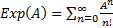 (Taylor series) and this series converges everywhere;
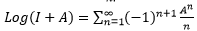 (Mercator series), converges with | A | <1 ;
 ;
; .
.
Efficient computation of the matrix exponent and the logarithm is a complex problem, and the most reasonable approach to its implementation is to use the corresponding mathematical library :).
Let's see what the Lie algebra matrices look like for some practically significant groups. For example, our simple group of rotations in the matrix form is written as “all 3x3 matrices with a single determinant”, and its corresponding Lie algebra consists of 3x3 matrices of the following form:
Where (x, y, z) is the aforementioned angular velocity vector, which determines the rotational speed according to the principle “vector length = angular velocity, direction = axis of rotation”. X, y, and z here can be considered as the kinematic equivalent of Euler angles — in essence, these are angular velocities of rotation relative to the x, y, and z axes. But in general, we get just another way of recording rotations in the axis and angle view.
If we consider the case of arbitrary motion in three-dimensional space, writing it down by 4x4 matrices of the form
, where R is a 3x3 rotation matrix, and T is a 3x1 shift vector, then the corresponding Lie algebra is obtained from matrices:Where (rx, ry, rz) has the already mentioned meaning of the vector of angular velocity, and (tx, ty, tz) is the vector of the instantaneous velocity of the body at the point (0,0,0). The corresponding pairs of vectors are called the motor of instantaneous velocities of a solid , and their use is associated with an elegant and relatively little-known mathematical apparatus of the so-called screw calculus , which deserves a separate article on Habré.
Want to add more scaling? Simply add diagonal elements (sx, sy, sz) , corresponding to the speed of "stretching" on each of the axes:
But for rigid body motion in 2D, which can be specified by 3x3 matrices, the Lie algebra is obtained from the matrices:
... and so on, I think you already caught the idea :). But anyway…
Why is all this necessary?
Interpolation
As a first example, let's take a simple 2D shape and try to move it in a continuous movement from one position to another. Parameterize the position of the model (x, y) and the angle of rotation (a) , perform linear interpolation ...
Everything seems to work, but there is some kind of weak, but clearly perceptible, unnatural movement. What is the matter? Let's draw the trajectories along which the points located initially on the left side of the screen move.
The lower part, where our airplane is located, is not too similar to a turn: different points move not only at different speeds, but also along different trajectories; however, the strangest thing happens in the upper left corner, where the points make a characteristic reciprocating motion. I did not do the corresponding illustration, because in practice such an artifact is not very common, but I think that among those who are engaged in three-dimensional animation, many have observed such a thing when interpolating at least a couple of times.
And what happens if we take the exhibitor instead? Let A be the matrix of the initial position of the object, and B be the matrix of the final position. We set the position of the object at time t as
where .As you can see, it turned out a clean smooth turn, in which all points of the object move at a constant speed. Of course, the same result could be achieved without resorting to the exponent, but simply remembering that any movement on a plane is either a parallel translation or a rotation around a certain point at a certain angle. It would be enough to choose the appropriate center of rotation and vary the angle. But the charm of the exponent and the logarithm is that it is an absolute no-brainer, only two or three lines of code that will work with the same success in all circumstances. Need to interpolate motion in 3D? The same formula will automatically give you a screw, even if you do not know the Shalya theorem. Need to interpolate linear motion? The same formula will give a linear transition.An interesting and useful by-property of exponentiation as an interpolation method is that when interpolating the transition between elements of a subgroup, the exponent “works” especially within this subgroup. That is, if, for example, you have a robot in three-dimensional space that can move only in a certain plane, or, say, rotates about a certain point, then the interpolation between its two positions will automatically occur only in the same plane or rotation relative to this points.rotates about a certain point, the interpolation between its two positions will automatically occur only in the same plane or rotation about this point.rotates about a certain point, the interpolation between its two positions will automatically occur only in the same plane or rotation about this point.
Parameterization and approximation
Another useful property follows from the fact that a properly defined Exp :
- always gives an element of the group of movements that we are interested in;
- decomposed into a taylor series.
Well, that is, let's say, we want to find a rotation matrix that will best meet a specific requirement. Let's say we have two pieces of the same surface, and we want to glue them together, for which we select the rotation matrix that best combines the first piece with the second one. To implement the search for such a matrix, we first need to somehow parametrize the space of these matrices. This can be done, for example, using the Euler angles, but when we substitute the resulting matrix with a bunch of sines and cosines, it will be unclear how to solve the resulting optimization problem. We can instead try using the elements of the motion matrix itself as parameters for optimization; this will result in a much simpler optimization problem (quadratic equation in the case of ICP),but there are no guarantees that the affine transformation matrix calculated in this way will be a rotation. There are several ways to circumvent this problem: for example, in a number of papers it is proposed to consider an affine matrix, and then orthogonalize it to the “nearest” rotation. Exponentiation provides one of the interesting alternatives. As mentioned at the beginning, Lie algebra is a much simpler “analog” of the Lie group (rotations) that interests us.Lie algebra is a much simpler “analog” of the Lie group (rotations) that interests us.Lie algebra is a much simpler “analog” of the Lie group (rotations) that interests us. Therefore:
- we parametrize elements of a Lie algebra (and this is the usual linear space);
- use the exhibitor to return to the group of interest.
At first glance, it may seem that this approach is even worse voiced at the beginning of the parameterization by Euler angles, since the matrix exponent in the optimization problem is even more inconvenient to consider than sines and cosines. However, for small movements, instead of the exponent, we can simply write its decomposition into a Taylor series:
For small A, this series converges very quickly (for arbitrarily large ones, it also converges, but slowly), by virtue of which it can simply be chopped off on the first or second term after the unit matrix. For example, extremely often for small angles use the approximation
It parameterizes the rotation matrix with a well-known approximation.
True, usually when this approximation is introduced, then neither the exhibitors nor the Taylor series are mentioned :). However, the “legs” of this approximation grow precisely from the Taylor series, and now you know how this approximation can be easily continued to 2, 3 and of any order for arbitrary classes of motions (and not just rotations). By the way, the well-known OpenCV-STAM is a special case for a group of three-dimensional rotations, the Rodriguez rotation formula .
The use of this kind of approximations allows us to simplify the optimization problem (for example, to reduce it again to a quadratic one) and does not require a dubious transition with solving the problem for affine matrices and the subsequent design of the result to the desired group. Its only limitation is the requirement for the smallness of the matrix A, but as a rule, to get around it is quite simple. It is enough just to parameterize not directly the “object position matrix”, but “the motion matrix to be applied to the object”. Provided that the object initially stands more or less somewhere in the right place, the necessary “shift” matrix in the whole class of tasks is quite small. For example, this approach works well in iterative algorithms, since the step of moving objects on each subsequent iteration into them, as a rule, decreases rapidly.
Here is such a simple, interesting and surprisingly little-known thing. Do you use matrix exponents and Lie algebras in your projects :)?
Source: https://habr.com/ru/post/306400/
All Articles