Working with the framework for iterative processing of graphs Giraph using RBM as an example

The indifferent by xetobyte
Hello. In the previous article, we described how to create your applications under the Giraph framework (an add-on to the Hadoop data processing system), and promised to consider in detail how to work with the Giraph, using the example of the Restricted Boltzmann Machine learning algorithm. So, at some point the group of segmentation of the audience of the department of advertising technologies Mail.Ru Group was faced with the need to choose a tool for quick analysis of graphs, and for a number of reasons (read below) our attention was attracted by the Apache Giraph system.
To understand how convenient this system is / performance / stable, etc., two participants of the Mail.Ru Technosphere laboratory, Alexander Shcherbakov and Pavel Kovalenko, were given the task of researching work with Giraph using the example of the Restricted Boltzmann Machine learning algorithm and trying to speed it up. On this task, the guys were able to better understand the subtleties of setting up Giraph and get practical experience working with open source projects.
Below, we will analyze in detail the implementation of the learning algorithm of the Boltzmann Machine (Restricted Boltzmann Machine, RBM) using the Giraph framework, which, in turn, is a superstructure over Hadoop. The main aspects of working with Giraph will be discussed, as well as some of the “chips” and methods of tuning the performance of this framework. You can read about the Giraph and how to create your first project on it in the previous article.
')
Article layout
1. RBM and Giraph
1.1. Brief description of RBM
1.2. Giraph
1.3. RBM and Giraph
2. Controlling the execution of compute-methods, worker context
2.1. Options to run
2.2. Overview of the wizard
2.3. Using WorkerContext and parameters stored in it in neurons
3. Overview of Initialization Classes
4. Description of the general class for neurons.
5. Classes of neurons
5.1. VisibleNeuronZero
5.2. HiddenNeuronFirst
5.3. VisibleNeuronFirst
5.4. NeuronDefault
5.5. VisibleNeuronLast
5.6. HiddenNeuronLast
5.7. VisibleNeuronOneStep
6. Overview of auxiliary classes
6.1. JSONWritable
6.2. RBMInputFormat
7. Optimization
7.1. Rib storage
7.2. Using vector operations
8. Future work
9. Conclusion
10. Literature
1. RBM and Giraph
1.1. Brief description of RBM
In this article, we will limit ourselves only to the facts that are necessary to understand what is happening. You can read more about RBM here or here
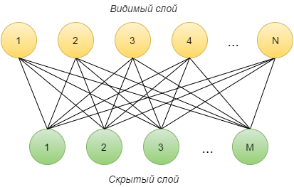
The Restricted Boltzmann Machine (RBM) is a neural network consisting of two layers: the visible and the hidden. Each visible neuron i is connected to each hidden j , and the initially connecting edge has a random weight w ij . Also, each neuron has an “offset” parameter (the visible layer is a i , the hidden layer is b i ). The number of neurons on the visible layer is denoted by N , on the hidden - M.
We describe how this network works.
- Let us take some vector v (0) from the training sample as the initial activation values of the neurons of the visible layer.
- On the hidden layer, the vector h (1) is considered as a linear combination of the values of the vector v (0) with weights w with the subsequent use of the sigmoidal activation function:
 where
where  - sigmoidal activation function. Further, h j = 1 with probability
  and 0 otherwise, in other words, we will sample.
 - Then, using the vector h (1), you can find the new value of the vector v (1) by the similar formulas:
 .
.
Steps 2–3 will be repeated k times. As a result, we obtain the vectors v (k) and h (k) .
A restricted Boltzmann machine can be considered as a method of nonlinear transformation of a feature space. We describe the initial vector v by the vector h according to the formulas presented above. According to the vector h, we can restore the original vector v with some accuracy. Thus, the vector v (k) is the result of applying k times the transform and restore operations to the vector v (0) . It is logical to require that the output vector v (k) be as close as possible to v (0) . This will mean that the vector x can be represented by the vector y with minimal loss of accuracy.
We will minimize the deviation of v (k) from v (0) by the method of back propagation of error . We divide the entire training sample into batches — subsamples of fixed size T. For each batch we will find the activation values, gradients and update the values of weights and offsets. Let the current batch consist of objects z i , i = 1 ... T. For each of them we find v (j) (z i ) and h (j) (z i ) , j = 1 ... k . Then we get [1, 2] the following formulas for changing network parameters:

where η is the learning rate.
One run of the algorithm for all batch will be called one epoch of training. To get the best result, it makes sense to conduct several ( K ) epochs of training so that each batch will be used K times to calculate gradients and update network parameters. In essence, we obtained an algorithm for stochastic gradient descent with respect to variables w , a, and b to minimize the mean for objects in the sample of the deviation of v (k) from v (0) .
1.2. Giraph
Giraph is an iterative processing system for large graphs that runs on top of the Hadoop distributed data processing system. We describe the main points in the work of this system. Giraph works with graphs. A graph is a set of vertices and a set of edges that connect these vertices. Counts are oriented and undirected. Technically, Giraph supports only directed graphs; to make an undirected graph, you need to create two edges between vertex A and B: from A to B and from B to A, with the same values.
Each vertex and each edge have their own values, and the values of the vertices and edges can be of different types (selected depending on the tasks). Each vertex contains a class that implements the
Computation interface and which describes the compute method. Calculations in Giraph are super superstep. At each super-step for the vertices, the compute method is called. Between supersteps vertices are delivered messages from other vertices, sent during the previous superstep. Messages have their own type, which does not have to match the types of vertices or edges.To coordinate the calculations, there is a special mechanism - MasterCompute (master). By default,
DefaultMaster is used in calculations - a class inherited from the abstract MasterCompute class. By itself, it is rather useless, since it does nothing (in many tasks nothing is required of it). Fortunately, there is an opportunity to make your own master, it must be inherited from MasterCompute , and the compute method must be implemented in it, which is performed before each super-step. The wizard allows you to select a class for the vertices, aggregate some data from the vertices and complete the calculations.Each vertex can be in two states: active and inactive. If the
voteToHalt() method is called inside the compute , then at the end of the super step, the vertex “falls asleep” - it becomes inactive at the next super step. Between supersteps vertices are delivered messages sent by other vertices in the course of superstep. All vertices that did not fall asleep at the previous super-step or received messages before the next are active and participate in the new super-step, performing their compute method. If all vertices are inactive, then the calculations end. At the end of the super step, the current state of the graph is saved to disk.The graph is processed on several workers (workers), the number of which does not change at run time. Each worker consistently processes several parts of the graph (Partition). The graph is divided into parts, which may change during processing. All this is done automatically and does not require user intervention.

Giraph uses the computational model vertex-oriented, in contrast to the same GraphX. This can be convenient for a number of tasks, since GraphX works with a graph as a simple set of parallel data, without paying attention to its structure. It is also worth noting that GraphX works with immutable graphs and requires Spark.
1.3. RBM and Giraph
And now let's correlate the received ideas about Giraph and RBM. There are vertices (neurons) connected by ribs. They are divided into two parts, which work in turn: the visible and hidden layer. One layer sends messages (activation values) to the other, making it active while falling asleep. Layers from time to time change the actions that they need to produce (this is work for the master). As we can see, RBM is nothing more than a bipartite undirected graph, and fits perfectly with the architecture of Giraph.
2. Controlling the execution of compute-methods, worker context
Let us understand how the work of our implementation of RBM is coordinated. First, we use our master, in which at each iteration we select the necessary class for the vertices. Secondly, a
WorkerContext is implemented - a class in which the current state of the network is calculated and from which the vertices can get the context of the running application. Thirdly, these are the parameters passed at startup. The master and context receive the values passed in the parameters.2.1. Options to run
To begin with, we note the parameters that can be set in our implementation:
maxEpochNumber- the number of training repetitions on all data;maxBatchNumber- the number of batches used for training;maxStepInSample- the number of runs of the batch from the visible layer to the hidden and back;learningRate- the pace of learning;visibleLayerSize- the number of neurons on the visible layer;hiddenLayerSize- the number of neurons on the hidden layer;inputPath- the path to the input files;useSampling- if true, performs sampling on a hidden layer.
2.2. Overview of the wizard
All parameters specified in clause 2.1 are used by the master to control the learning process. Let us consider in more detail how this happens.

First, a visible layer is created. It is configured by the
VisibleInitialize class. Then the same thing happens for the hidden layer with the class HiddenInitialize . Once the network is created, you can start learning. It consists of several eras. The epoch, in turn, is a consistent learning on this set of batches. Thus, in order to understand how the whole learning process takes place, it is necessary to understand learning in one batch.
In general, the training takes place as follows (scheme 1):
- Reading data in a visible layer.
- Preservation of a positive gradient value by a hidden layer.
- Maintaining a positive gradient value in a visible layer.
- Calculating the activation value of the hidden layer.
- Calculate the activation value of the visible layer.
- Calculating the activation value of the hidden layer.
- Repeat steps 5 and 6 more (
maxStepInSample- 3) times. - Update weights of outgoing edges of the visible layer.
- Update scales on a hidden layer.
It is worth noting that the activation values are considered at all steps except the 1st and 9th. Total will be executed
(maxStepInSample + 1) * 2 steps.
In the case when we send data to the hidden layer only once (
maxStepInSample = 1), the scheme changes somewhat (scheme 2):- Reading data in a visible layer.
- Preservation of a positive gradient value by a hidden layer.
- Update weights of outgoing edges of the visible layer.
- Update scales on a hidden layer.
Activation values in this variant are recalculated only on the 2nd and 3rd steps. Thus, we have seven classes for neurons (graph vertices) used in the learning process:
| Class name | Purpose | Relevant Steps | |
| From scheme 1 | From scheme 2 | ||
VisibleNeuronZero | The zero stage of learning with reading data also preserves the positive part of the gradient for offsets | one | one |
VisibleNeuronFirst | Preserves the positive part of the gradient in the visible layer | 3 | - |
VisibleNeuronLast | The last step of the training on the visible layer, considers the negative part of the gradient and updates the weights of the edges emerging from the visible layer. | eight | - |
VisibleNeuronOneStep | The combination of classes VisibleNeuronFirst and VisibleNeuronLast , is used in the case when maxStepInSample = 1 | - | 3 |
HiddenNeuronFirst | Saves a positive gradient value for the hidden layer (only for offsets b , weights gradients w are calculated on the visible layer) | 2 | 2 |
HiddenNeuronLast | Updates the weights of ribs emerging from the hidden layer. | 9 | four |
NeuronDefault | Called both on the visible layer and on the hidden layer and simply recalculates the activation values. | 4, 5, 6 | - |
2.3. Using WorkerContext and parameters stored in it in neurons
In order for the neurons to use the transmitted parameters, they made their own WorkerContext, which, firstly, transmits information about the size of the layers during initialization, secondly, gives the neurons information about the pace of learning, whether it is necessary to do sampling and data paths. In this class, regardless of the master, it is calculated which class is currently used for neurons.
3. Overview of Initialization Classes
Once again, but in more detail we will stop on how the graph is initialized. The application starts with a single dummy top. It performs
compute from InitialNode . The only thing that happens in this class is sending out empty messages to vertices with id from 1 to visibleLayerSize (vertices with these identifiers are immediately created and used in the next step). Immediately after this, the vertex goes to sleep (a voteToHalt call) and is never used again.Before the next step, MasterCompute sets
VisibleInitialize as the compute class, so the vertices created as a result of sending the message will execute it. First, the vertex generates edges going out of it with random weights to the vertices with the id from –hiddenLayerSize to –1. Then these weights are sent to the corresponding vertices of the hidden layer (recall that this causes the creation of these vertices). And at the end of each vertex a zero offset is added. After that, the visible layer "falls asleep", since its creation is complete.At the last stage of initialization, the compute of
HiddenInitialize is executed in the neurons of the hidden layer. Each vertex is iterated by the messages that came to it and creates the corresponding edges. Thus, each connection between neurons is defined by two edges with the same weights. Next, create a zero offset. Then the hidden layer “wakes up” visible with empty messages, and “falls asleep” itself.
4. Description of the general class for neurons.
Classes of neurons in many respects perform very similar actions that can be meaningfully combined into a set of various functions. The difference lies in the fact that in some classes certain functions are called / not called. Those functions that are called in all classes of neurons were allocated to a separate abstract class
NeuronCompute . All classes of neurons are inherited from it, and compute functions are implemented in them, in which both NeuronCompute methods and methods specific to a particular class can be called. And here, actually, and the list of the functions realized in it:sigma- returns the value of the sigma function from the passed parameter;ComputeActivateValues- returns the activation values for the batch according to the activation values received in the messages and the vertex offset;SendActivateValues- sends activation values to outgoing edges;ComputePositivePartOfBiasGradient- returns the positive part of the gradient for offsets;UpdateBiases- updates the offset;AddBias- adds zero offset to the vertex;SendNewEdges- sends new edge values to the hidden layer.
5. Classes of neurons
We describe the classes that implement neurons. Depending on the number of superstep selected one or another class.
5.1. VisibleNeuronZero
This class is the first in the era. It contains two proprietary methods:
ReadBatch and compute . It is easy to guess that in the ReadBatch method the next batch is loaded. The number of the batch and the path are taken from the WorkerContext. /** * */ double[] activateValues; double positiveBias; activateValues = ReadBatch(vertex); // . WorkerContext' positiveBias = ComputePositivePartOfBiasGradient(activateValues); // SendActivateValues(vertex, activateValues); // /** * */ JSONWritable value = vertex.getValue(); value.addDouble("Positive bias", positiveBias); value.addArray("Value", activateValues); vertex.setValue(value); vertex.voteToHalt(); // 5.2. HiddenNeuronFirst
This is the first class running on a hidden layer. It consists entirely of methods of the
NeuronCompute class. Take a look at his compute : /** * */ double bias = vertex.getValue().getDouble("Bias"); double[] activateValues; double positiveBias; activateValues = ComputeActivateValues(vertex, messages, bias); // positiveBias = ComputePositivePartOfBiasGradient(activateValues); // SendActivateValues(vertex, activateValues); // /** * */ JSONWritable value = vertex.getValue(); value.addDouble("Positive bias", positiveBias); value.addArray("Value", activateValues); vertex.setValue(value); vertex.voteToHalt(); // 5.3. VisibleNeuronFirst
Now that we have activation values for the visible and hidden layer, we can calculate the positive part of the gradient for the edges.
/** * */ double bias = vertex.getValue().getDouble("Bias"); double[] activateValues = vertex.getValue().getArray("Value"); HashMap<Long, Double> positiveGradient; ArrayList valueAndGrad = ComputeActivateValuesAndPositivePartOfGradient(vertex, messages, activateValues, bias); // activateValues = (double[])valueAndGrad.get(0); positiveGradient = (HashMap<Long, Double>)valueAndGrad.get(1); SendActivateValues(vertex, activateValues); // /** * */ JSONWritable value = vertex.getValue(); value.addArray("Value", activateValues); value.addHashMap("Positive gradient", positiveGradient); vertex.setValue(value); vertex.voteToHalt(); // 5.4. NeuronDefault
This class is common to both layers. Here is his compute:
/** * */ double bias = vertex.getValue().getDouble("Bias"); double[] activateValues; activateValues = ComputeActivateValues(vertex, messages, bias); // SendActivateValues(vertex, activateValues); // /** * */ JSONWritable value = vertex.getValue(); value.addArray("Value", activateValues); vertex.setValue(value); vertex.voteToHalt(); // 5.5. VisibleNeuronLast
This is the last stage, performed on the visible layer, and it is in it that the weights are updated. It would all end there (as in successive implementations), but you also need to update the edges, directed in the opposite direction.
/** * */ double bias = vertex.getValue().getDouble("Bias"); double[] activateValues = vertex.getValue().getArray("Value"); double positiveBias = vertex.getValue().getDouble("Positive bias"); activateValues = ComputeGradientAndUpdateEdges(vertex, messages, activateValues.length, bias); // . bias = UpdateBiases(activateValues, bias, positiveBias); // SendNewEdges(vertex); // /** * */ JSONWritable value = vertex.getValue(); value.addArray("Value", activateValues); value.addDouble("Bias", bias); vertex.setValue(value); vertex.voteToHalt(); // 5.6. HiddenNeuronLast
At this step, we take the new edge weights from the messages and set them on the existing edges.
/** * */ double bias = vertex.getValue().getDouble("Bias"); double[] activateValues = vertex.getValue().getArray("Value"); double positiveBias = vertex.getValue().getDouble("Positive bias"); UpdateEdgesByMessages(vertex, messages); // bias = UpdateBiases(activateValues, bias, positiveBias); // /** * */ JSONWritable value = vertex.getValue(); value.addDouble("Bias", bias); vertex.setValue(value); vertex.voteToHalt(); // 5.7. VisibleNeuronOneStep
This class is used in the case when one pass of activation values to the hidden layer and back is performed. It combines the functionality of the classes VisibleNeuronFirst and VisibleNeuronLast.
/** * */ double bias = vertex.getValue().getDouble("Bias"); double[] activateValues = vertex.getValue().getArray("Value"); double positiveBias = vertex.getValue().getDouble("Positive bias"); activateValues = ComputeGradientAndUpdateEdges(vertex, messages, activateValues, bias); // bias = UpdateBiases(activateValues, bias, positiveBias); // SendNewEdges(vertex); // /** * */ JSONWritable value = vertex.getValue(); value.addArray("Value", activateValues); value.addDouble("Bias", bias); vertex.setValue(value); vertex.voteToHalt(); // 6. Description of auxiliary classes
6.1. JSONWritable
JSONWritable - the class that we use as a class for the value at the vertices and for the messages to be sent. In essence, this is a Writable wrapper for a JSON object. This data storage format is convenient because the type and number of values that need to be stored vary depending on the current iteration. Google GSON is used as a library for working with JSON. For recording and sending, the JSON string is wrapped in an object of the Text class.For the Writable class, the main methods are
readFieds — read an object of this class from the input stream and write — write the object to the output stream. Below is their implementation for the JSONWritable class. public class JSONWritable implements Writable { private JsonElement json; public void write(DataOutput out) throws IOException { Text text = new Text(this.json.toString()); text.write(out); } public void readFields(DataInput in) throws IOException { Text text = new Text(); text.readFields(in); JsonParser parser = new JsonParser(); this.json = parser.parse(text.toString()); } /* */ } Since it was necessary to store a lot of different data in the JSON object, it is convenient to present it as a dictionary with string keys (Bias, PositiveGradient, etc.). For this task, it was necessary to write some complex objects in JSON, including at the vertices it is necessary to store the positive part of the gradient for the edges. It is represented as a HashMap, the keys of which are the id vertices of the destination edges (of the long type), and the values are the positive part of the gradient of the corresponding edge (of the double type). To do this,
JSONWritable has written special methods for adding and extracting a HashMap by key. public HashMap getHashMap(String key) { HashMap a = new HashMap(); Iterator it = this.json.getAsJsonObject().getAsJsonObject(key).entrySet().iterator(); while (it.hasNext()) { Map.Entry me = (Map.Entry) it.next(); a.put(Long.valueOf(me.getKey().toString()), ((JsonElement) me.getValue()).getAsDouble()); } return a; } public void addHashMap(String key, HashMap a) { Iterator it = a.entrySet().iterator(); JsonObject obj = new JsonObject(); while (it.hasNext()) { Map.Entry me = (Map.Entry) it.next(); obj.addProperty(me.getKey().toString(), (double) me.getValue()); } this.json.getAsJsonObject().add(key, obj); } 6.2. RBMInputFormat
This class is used to read the graph written to the file. It is a modification of the standard JsonLongDoubleFloatDoubleVertexInputFormat to work with other data types. Input data should be written in the following form: each line of the input file is a JSON list corresponding to one vertex. Each list is written in the format
[Id_, __, _] , where Id is an integer, [[Id__, __], … ] .7. Optimization
Many of Giraph's work parameters, such as the method of storing edges and messages, the method of splitting vertices between workers, the level of debug output and the settings of counters, can be configured at startup from the command line. A complete list of startup options can be found at http://giraph.apache.org/options.html . Setting these options for a specific task allows you to achieve a noticeable increase in performance.
7.1. Rib storage
In Giraph, the edges are stored by default as a byte array (ByteArray) and are de-serialized every time they are accessed. This helps save memory, but increases the running time. To speed up the program, we tried to store the edges in the form of a list (ArrayList) and in the form of a dictionary, the keys in which are the final vertices of the edges (HashMap). The list allows you to quickly iterate over the edges, while the dictionary allows you to quickly find an edge along its top of the destination.
— Giraph, ,
-ca giraph.outEdgesClass=org.apache.giraph.edge.ArrayListEdges ( ).: 800 , 150 , 50 , 100 , (
maxStepInSample=2 ), , 6 . . , , , , ( 2—4), 20%.
7.2.
. . , . . , , smile , .
, . .

8.
— . , , Hive — HDFS SQL- .
9. Future work
, Giraph — , , RBM. , / . , Giraph. , .
10.
- RBM
- Giraph'
- Smile
- Claudio Martella, Roman Shaposhnik, Dionysios Logothetis. Practical Graph Analytics with Apache Giraph. 2015
- RBM Giraph
Source: https://habr.com/ru/post/306362/
All Articles