A little bit about designing self-timed circuits
The forums on electronics periodically recall self-timed circuits, but very few people understand what it is all about, what self-synchronous circuitry has useful properties, and what disadvantages they have. The short text below will allow the reader to get acquainted with the basics of the synthesis of the simplest self-timed circuits, and try to design them yourself.
At the beginning of a few introductory words. Asynchronous, you can call any scheme without external clocking. In this case, various types of asynchronous circuits use a different principle of operation, and self-timed circuits are just one of their varieties. Under the self-timed usually understand the so-called. semi-modular schemes, due to the possibility of their representation in the form of algebraic structures that make up semi-modular lattices (forgive me for mathematics for possible inaccuracies). One of the features of semi-modular (read-self-synchronous) circuits is independence from delays, which in practice means that the circuit works in all conditions under which transistors are capable of switching. However, no one bothers to design self-timed circuits on mechanical relays or any other switches. It is no secret that it is very difficult to develop such schemes, but they are not threatened by failure due to overheating, for example, or the effects of aging.
With the introduction of everything, and you can proceed to practice. According to the design method, all self-timed circuits can be divided into two groups - control automata, and circuits with a large number of logic. Where does this separation come from? Automatic control, it is simple devices like counters, latches, triggers, or some small controllers. These devices are mainly designed manually using Petri nets (graph language describing parallel dynamic processes), and then synthesized in Petrify or other tools. The schemes with a large number of logic should be understood as familiar to all the nodes of computing devices: controllers, peripherals, PDP, arithmetic units, and anything else that uses multiplication, addition, comparison, multiplexing, etc. Such schemes are too complicated to be described by Petri nets, and are designed differently (this is the topic of a separate cycle of publications, or even a whole textbook). Therefore, we start with the basics, with Petri nets.
Take for example the simplest self-timed counting trigger. Like all self-timed circuits, it works on the same principle as the ring oscillator on inverters:
')
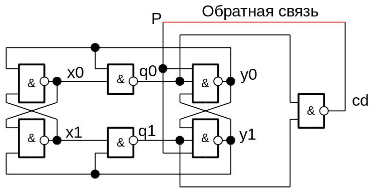
The signal P is counting, the signals x0, x1, y0, y1 are internal, the pair { q0, q1 } are the output signals of the counter, and cd is the indicator of the end of transients in the circuit. If the cd signal is closed to the counting input P , the machine will work indefinitely. Anyone who wishes can be convinced of this with the help of the usual modeling:
Please note that the logic elements must have a non-zero delay, and the circuit requires an initial installation. In the gland (if someone tries to make this scheme on the FPGA or placer) the initial installation is not required.
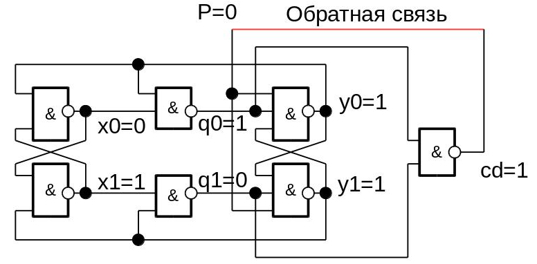
And now let's do reverse engineering to understand how to get a counting trigger scheme using Petri nets. Choose an arbitrary initial arrangement of values at the outputs of the elements (you can take from the simulation, or come up with yourself):
Since P = cd , the value of P in the next moment of time should change by 1. Construct a graph, at the vertices of which there will be variables, and edges - the direction of switching of variables. We mark the variables with the + sign if they switch from 0 to 1, and with the minus sign if they switch from 1 to 0. Enter the graph in the Workcraft editor (you can download it for free from http://www.workcraft.org . Select the File - Create work - Signal Transition Graph, and enter the graph). The initial switching of the signal P from 0 to 1 (ie, P +) will be marked with an incoming arrow with a circle (token). The graph will turn out:
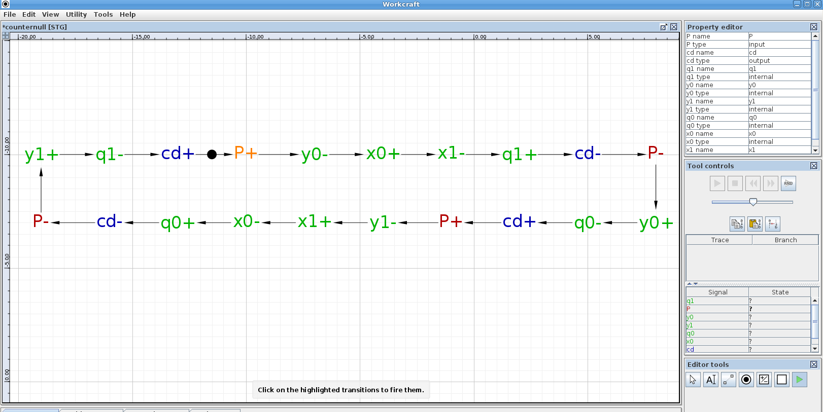
After switching P to 1, the signal goes to y0 to 0, then x0 to 1, and so on, until we return to the beginning. As can be seen from the graph, the output variables { q1, q0 } switch in a cycle of 10-11-01-11-10-11 , etc., which corresponds to the operation of the counting trigger. You can turn on the Petri network simulator mode. To do this, click on the green triangle icon in the lower right window of the Editor Tools window, and then run the simulation in the Tool Controls window that appears above.
The next step is graph synthesis in Petrify. Select Tools - Synthesis - Complex gate synthesis [Petrify] in the menu, and get the log:
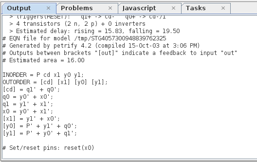
The synthesis was successful (which means that the scheme issemi - modular self-synchronous), and the formulas obtained correspond to the original scheme. Reverse engineering successfully completed.
From the graph it becomes obvious that the operability of the counting trigger does not depend on the delays: wherever you add a delay to the circuit, it only slows down its work, but does not change the order of switching elements and does not violate the logic of the circuit.
The described procedures (in order: from graph to scheme) allow to synthesize and check for self-synchronization only the schemes of latches, triggers, counters, or arbitrary controllers, whose behavior is described by the Petri net containing no more than 50 variables. More complex schemes cannot be developed in this way (it is necessary to use other design approaches). But to learn the basics of developing self-timed circuits, the considered example of a counting trigger (as well as tutorials from the workcraft distribution) is the very thing. Interested in theory, I recommend reading the textbook on Petri nets and self-timed circuits: Marakhovsky V. B., Rozenblyum L. Ya., Yakovlev A. V. Simulation of parallel processes. Petri nets , as well as to study the material on the workcraft developers website .
At the beginning of a few introductory words. Asynchronous, you can call any scheme without external clocking. In this case, various types of asynchronous circuits use a different principle of operation, and self-timed circuits are just one of their varieties. Under the self-timed usually understand the so-called. semi-modular schemes, due to the possibility of their representation in the form of algebraic structures that make up semi-modular lattices (forgive me for mathematics for possible inaccuracies). One of the features of semi-modular (read-self-synchronous) circuits is independence from delays, which in practice means that the circuit works in all conditions under which transistors are capable of switching. However, no one bothers to design self-timed circuits on mechanical relays or any other switches. It is no secret that it is very difficult to develop such schemes, but they are not threatened by failure due to overheating, for example, or the effects of aging.
With the introduction of everything, and you can proceed to practice. According to the design method, all self-timed circuits can be divided into two groups - control automata, and circuits with a large number of logic. Where does this separation come from? Automatic control, it is simple devices like counters, latches, triggers, or some small controllers. These devices are mainly designed manually using Petri nets (graph language describing parallel dynamic processes), and then synthesized in Petrify or other tools. The schemes with a large number of logic should be understood as familiar to all the nodes of computing devices: controllers, peripherals, PDP, arithmetic units, and anything else that uses multiplication, addition, comparison, multiplexing, etc. Such schemes are too complicated to be described by Petri nets, and are designed differently (this is the topic of a separate cycle of publications, or even a whole textbook). Therefore, we start with the basics, with Petri nets.
Take for example the simplest self-timed counting trigger. Like all self-timed circuits, it works on the same principle as the ring oscillator on inverters:
')
The signal P is counting, the signals x0, x1, y0, y1 are internal, the pair { q0, q1 } are the output signals of the counter, and cd is the indicator of the end of transients in the circuit. If the cd signal is closed to the counting input P , the machine will work indefinitely. Anyone who wishes can be convinced of this with the help of the usual modeling:
Netcode with testbench source code
`timescale 1ns/10ps module sim(); wire P,cd; counter dut(.P(P), .cd(cd)); assign P = cd; initial begin force P=0; force dut.x0=0; force dut.x1=1; #2; release P; release dut.x1; release dut.x0; end endmodule module counter( input wire P, output wire cd ); wire x0, x1, y0, y1, q0, q1; nand2 U1 (.A(y0), .B(x1), .Y(x0)); nand2 U2 (.A(y1), .B(x0), .Y(x1)); nand2 U3 (.A(y0), .B(x0), .Y(q0)); nand2 U4 (.A(y1), .B(x1), .Y(q1)); nand3 U5 (.A(P), .B(q0), .C(y1), .Y(y0)); nand3 U6 (.A(P), .B(q1), .C(y0), .Y(y1)); nand2 U7 (.A(q0), .B(q1), .Y(cd)); endmodule module nand2( input wire A, B, output wire Y ); assign #1 Y = ~(A & B); endmodule module nand3( input wire A, B, C, output wire Y ); assign #1 Y = ~(A & B & C); endmodule Please note that the logic elements must have a non-zero delay, and the circuit requires an initial installation. In the gland (if someone tries to make this scheme on the FPGA or placer) the initial installation is not required.
And now let's do reverse engineering to understand how to get a counting trigger scheme using Petri nets. Choose an arbitrary initial arrangement of values at the outputs of the elements (you can take from the simulation, or come up with yourself):
Since P = cd , the value of P in the next moment of time should change by 1. Construct a graph, at the vertices of which there will be variables, and edges - the direction of switching of variables. We mark the variables with the + sign if they switch from 0 to 1, and with the minus sign if they switch from 1 to 0. Enter the graph in the Workcraft editor (you can download it for free from http://www.workcraft.org . Select the File - Create work - Signal Transition Graph, and enter the graph). The initial switching of the signal P from 0 to 1 (ie, P +) will be marked with an incoming arrow with a circle (token). The graph will turn out:
After switching P to 1, the signal goes to y0 to 0, then x0 to 1, and so on, until we return to the beginning. As can be seen from the graph, the output variables { q1, q0 } switch in a cycle of 10-11-01-11-10-11 , etc., which corresponds to the operation of the counting trigger. You can turn on the Petri network simulator mode. To do this, click on the green triangle icon in the lower right window of the Editor Tools window, and then run the simulation in the Tool Controls window that appears above.
The next step is graph synthesis in Petrify. Select Tools - Synthesis - Complex gate synthesis [Petrify] in the menu, and get the log:
The synthesis was successful (which means that the scheme is
From the graph it becomes obvious that the operability of the counting trigger does not depend on the delays: wherever you add a delay to the circuit, it only slows down its work, but does not change the order of switching elements and does not violate the logic of the circuit.
The described procedures (in order: from graph to scheme) allow to synthesize and check for self-synchronization only the schemes of latches, triggers, counters, or arbitrary controllers, whose behavior is described by the Petri net containing no more than 50 variables. More complex schemes cannot be developed in this way (it is necessary to use other design approaches). But to learn the basics of developing self-timed circuits, the considered example of a counting trigger (as well as tutorials from the workcraft distribution) is the very thing. Interested in theory, I recommend reading the textbook on Petri nets and self-timed circuits: Marakhovsky V. B., Rozenblyum L. Ya., Yakovlev A. V. Simulation of parallel processes. Petri nets , as well as to study the material on the workcraft developers website .
Source: https://habr.com/ru/post/306056/
All Articles