Visualization of Euro 2016 statistics using Python and Inkscape

Hi, Habr!

A little more than a week has passed since the end of the European Championship 2016 in France. This championship will be remembered for us by the unsuccessful performance of the Russian national team, shown by the will of the Icelandic national team, the amazing game of the national teams of France and Portugal. In this article, we will work with the data, build several graphs and edit them in the Inkscape vector editor. Who cares - I ask under the cat.

Content

Work with API data
Data Visualization with Python
Editing vector graphics in Inkscape

1. Work with API data

To visualize football data, you must first obtain it. For these purposes, we will use the API football-data.org . The following methods are available to us:

List of competitions - "api.football-data.org/v1/competitions/?season={year}"
The list of teams (by competition identifier) - “api.football-data.org/v1/competitions/{competition_id}/teams”
List of matches (by competition ID) - “api.football-data.org/v1/competitions/{competition_id}/fixtures”
Team information - "api.football-data.org/v1/teams/{team_id}"
List of players (by team ID) - "api.football-data.org/v1/teams/{team_id}/players"

Details on all methods are in the API documentation.
Let's now try to work with the data. To begin, let's try to study the structure of the returned data for the competitions method (list of competitions):

[{'_links': {'fixtures': {'href': 'http://api.football-data.org/v1/competitions/424/fixtures'}, 'leagueTable': {'href': 'http://api.football-data.org/v1/competitions/424/leagueTable'}, 'self': {'href': 'http://api.football-data.org/v1/competitions/424'}, 'teams': {'href': 'http://api.football-data.org/v1/competitions/424/teams'}}, 'caption': 'European Championships France 2016', 'currentMatchday': 7, 'id': 424, 'lastUpdated': '2016-07-10T21:32:20Z', 'league': 'EC', 'numberOfGames': 51, 'numberOfMatchdays': 7, 'numberOfTeams': 24, 'year': '2016'}, {'_links': {'fixtures': {'href': 'http://api.football-data.org/v1/competitions/426/fixtures'}, 'leagueTable': {'href': 'http://api.football-data.org/v1/competitions/426/leagueTable'}, 'self': {'href': 'http://api.football-data.org/v1/competitions/426'}, 'teams': {'href': 'http://api.football-data.org/v1/competitions/426/teams'}}, 'caption': 'Premiere League 2016/17', 'currentMatchday': 1, 'id': 426, 'lastUpdated': '2016-06-23T10:42:02Z', 'league': 'PL', 'numberOfGames': 380, 'numberOfMatchdays': 38, 'numberOfTeams': 20, 'year': '2016'},

Before we start working with Python, we need to make the necessary imports:

 import datetime import random import re import os import requests import json import pandas as pd import numpy as np import matplotlib.pyplot as plt from matplotlib import rc pd.set_option('display.width', 1100) plt.style.use('bmh') DIR = os.path.dirname('__File__') font = {'family': 'Verdana', 'weight': 'normal'} rc('font', **font)

The data structure is understandable, we will try to upload data about the competition for the 2015-2016 year in pandas.DataFrame. In parallel, we will save data that we will work with in .csv files, since only 50 API requests per day can be made for free. Restrictions are also imposed on the time period of the data - only 2015-2016 years are available to us for free.

 competitions_url = 'http://api.football-data.org/v1/competitions/?season={year}' data = [] for y in [2015, 2016]: response = requests.get(competitions_url.format(year=y)) competitions = json.loads(response.text) competitions = [{'caption': c['caption'], 'id': c['id'], 'league': c['league'], 'year': c['year'], 'games_count': c['numberOfGames'], 'teams_count': c['numberOfTeams']} for c in competitions] COMP = pd.DataFrame(competitions) data.append(COMP) COMP = pd.concat(data) COMP.to_csv(os.path.join(DIR, 'input', 'competitions_2015_2016.csv')) COMP.head(20)

Fine! We see the European Championship 2016 in the list:

	caption	games_count	id	league	teams_count	year
12	League One 2015/16	552	425	EL1	24	2015
0	European Championships France 2016	51	424	EC	24	2016

Now we can get a list of teams by the identifier (id) of these competitions - we use the teams method to get the list of teams of Euro 2016.

 teams_url = 'http://api.football-data.org/v1/competitions/{competition_id}/teams' response = requests.get(teams_url.format(competition_id=424)) teams = json.loads(response.text)['teams'] teams = [dict(code=team['code'], name=team['name'], flag_url=team['crestUrl'], players_url=team['_links']['players']['href']) for team in teams] TEAMS = pd.DataFrame(teams) TEAMS.to_csv(os.path.join(DIR, 'input', 'teams_euro2016.cvs')) TEAMS.head(24)

	code	flag_url	name	players_url
0	Fra	upload.wikimedia.org/wikipedia/en/c/c3 ...	France	api.football-data.org/v1/teams/773/players
one	ROU	upload.wikimedia.org/wikipedia/commons ...	Romania	api.football-data.org/v1/teams/811/players
2	ALB	upload.wikimedia.org/wikipedia/commons ...	Albania	api.football-data.org/v1/teams/1065/pla ...
3	SUI	upload.wikimedia.org/wikipedia/commons ...	Switzerland	api.football-data.org/v1/teams/788/players
four	WAL	upload.wikimedia.org/wikipedia/commons ...	Wales	api.football-data.org/v1/teams/833/players

The structure of our table is a table (DataFrame) with the following columns:

code (three digit country code)
flag_url (link to the .svg file of the country flag in our case, and in the original crestUrl, the .svg file of the team symbol)
name (command name)
players_url (link to the API page with player data - for some reason there is no player data for the national teams, perhaps this is another API restriction)

In our subsequent work, we will also need .svg command flag files - just download them to a separate directory, I did it quickly and easily using the Chrono extension for Chrome.

Now let's try to get data directly about the matches of Euro 2016. First, let's look at the structure of the server response for the selected “orders” method. For example, let us analyze the structure of information about a match that ends with a penalty shootout (this is the most complex composition of data from possible for this method).

 games_url = 'http://api.football-data.org/v1/competitions/{competition_id}/fixtures' response = requests.get(games_url.format(competition_id=424)) games = json.loads(response.text)['fixtures'] #       ,   . games_selected = [game for game in games if 'extraTime' in game['result']] games_selected[0]

In the answer we get the following:

 {'_links': {'awayTeam': {'href': 'http://api.football-data.org/v1/teams/794'}, 'competition': {'href': 'http://api.football-data.org/v1/competitions/424'}, 'homeTeam': {'href': 'http://api.football-data.org/v1/teams/788'}, 'self': {'href': 'http://api.football-data.org/v1/fixtures/150457'}}, 'awayTeamName': 'Poland', 'date': '2016-06-25T13:00:00Z', 'homeTeamName': 'Switzerland', 'matchday': 4, 'result': {'extraTime': {'goalsAwayTeam': 1, 'goalsHomeTeam': 1}, 'goalsAwayTeam': 1, 'goalsHomeTeam': 1, 'halfTime': {'goalsAwayTeam': 1, 'goalsHomeTeam': 0}, 'penaltyShootout': {'goalsAwayTeam': 5, 'goalsHomeTeam': 4}}, 'status': 'FINISHED'}

To make it easier to work with the data and the process of loading them into the DataFrame, we will write a small function that accepts a dictionary with information about the match as an attribute and returns a dictionary of a type convenient for us.

Match dictionary processing function

 def handle_game(game): date = game['date'] team_1 = game['homeTeamName'] team_2 = game['awayTeamName'] matchday = game['matchday'] team_1_goals_main = game['result']['goalsHomeTeam'] team_2_goals_main = game['result']['goalsAwayTeam'] status = game['status'] if 'extraTime' in game['result']: team_1_goals_extra = game['result']['extraTime']['goalsHomeTeam'] team_2_goals_extra = game['result']['extraTime']['goalsAwayTeam'] if 'penaltyShootout' in game['result']: team_1_goals_penalty = game['result']['penaltyShootout']['goalsHomeTeam'] team_2_goals_penalty = game['result']['penaltyShootout']['goalsAwayTeam'] else: team_1_goals_penalty = team_2_goals_penalty = 0 else: team_1_goals_extra = team_2_goals_extra = team_1_goals_penalty = team_2_goals_penalty = 0 team_1_goals = team_1_goals_main + team_1_goals_extra team_2_goals = team_2_goals_main + team_2_goals_extra if (team_1_goals + team_1_goals_penalty) > (team_2_goals + team_2_goals_penalty): team_1_win = 1 team_2_win = 0 draw = 0 elif (team_1_goals + team_1_goals_penalty) < (team_2_goals + team_2_goals_penalty): team_1_win = 0 team_2_win = 1 draw = 0 else: team_1_win = team_2_win = 0 draw = 1 game = dict(date=date, team_1=team_1, team_2=team_2, matchday=matchday, status=status, team_1_goals=team_1_goals, team_2_goals=team_2_goals, team_1_goals_extra=team_1_goals_extra, team_2_goals_extra=team_2_goals_extra, team_1_win=team_1_win, team_2_win=team_2_win, draw=draw, team_1_goals_penalty=team_1_goals_penalty, team_2_goals_penalty=team_2_goals_penalty) return game #           game = handle_game(games_selected[0]) print(game)

Here is the returned dictionary:

 {'date': '2016-06-25T13:00:00Z', 'draw': 0, 'matchday': 4, 'status': 'FINISHED', 'team_1': 'Switzerland', 'team_1_goals': 2, 'team_1_goals_extra': 1, 'team_1_goals_penalty': 4, 'team_1_win': 0, 'team_2': 'Poland', 'team_2_goals': 2, 'team_2_goals_extra': 1, 'team_2_goals_penalty': 5, 'team_2_win': 1}

Now we are ready to load data on all matches of Euro 2016 in the DataFrame.

 games_url = 'http://api.football-data.org/v1/competitions/{competition_id}/fixtures' response = requests.get(games_url.format(competition_id=424)) games = json.loads(response.text)['fixtures'] GAMES = pd.DataFrame([handle_game(g) for g in games]) GAMES.to_csv(os.path.join(DIR, 'input', 'games_euro2016.csv')) GAMES.head()

	date	draw	matchday	status	team_1	team_1_goals	team_1_goals_extra	team_1_goals_penalty	team_1_win	team_2	team_2_goals	team_2_goals_extra	team_2_goals_penalty	team_2_win
0	2016-06-10T19: 00: 00Z	0	one	FINISHED	France	2	0	0	one	Romania	one	0	0	0
one	2016-06-11T13: 00: 00Z	0	one	FINISHED	Albania	0	0	0	0	Switzerland	one	0	0	one

Well, the data is loaded into the DataFrame, but this structure is not suitable for data analysis. Guided by the principles of the document “Tidy Data, Hadley Wickham (2014)”, we will adjust the structure of the DataFrame so that one variable (command) is identical to one line - in fact, we will double the number of lines in the Dataframe. Also, adjust the column names to make it easier to work with.

 #         . GAMES['date'] = pd.to_datetime(GAMES.date) #            () GAMES = GAMES.reindex(columns=['date', 'matchday', 'status', 'team_1', 'team_1_win', 'team_1_goals', 'team_1_goals_extra', 'team_1_goals_penalty', 'team_2', 'team_2_win', 'team_2_goals', 'team_2_goals_extra', 'team_2_goals_penalty', 'draw']) new_columns = ['date', 'mday', 'status', 't1', 't1w', 't1g', 't1ge', 't1gp', 't2', 't2w', 't2g', 't2ge', 't2gp', 'draw'] GAMES.columns = new_columns GAMES.head() #    DataFrame #   DataFrame  ,  ,      DataFrame. GAMES_2 = GAMES.ix[:,[0, 1, 2, 8, 9, 10, 11, 12, 3, 4, 5, 6, 7, 13]] GAMES_2.columns = new_columns GAMES_F = pd.concat([GAMES, GAMES_2]) GAMES_F.sort(['date'], inplace=True) GAMES_F.head()

	date	mday	status	t1	t1w	t1g	t2	t2w	t2g
0	2016-06-10 19:00:00	one	FINISHED	France	one	2	Romania	0	one
0	2016-06-10 19:00:00	one	FINISHED	Romania	0	one	France	one	2
one	2016-06-11 13:00:00	one	FINISHED	Albania	0	0	Switzerland	one	one

This structure is much better, but for further work we will need a few more minor changes.

 #           - "g" -  -     GAMES_F['g'] = GAMES_F.t1g + GAMES_F.t2g GAMES_F['idx'] = GAMES_F.index #              . #  ,     51,   15  -,  -  . #      DataFrame TP = pd.DataFrame({'typ': ['']*36 + ['1/8']*8 + ['1/4']*4 + ['1/2']*2 + ['']*1, 'idx': range(0, 51)}) #   DataFrame GAMES_F= pd.merge(GAMES_F, TP, how='left', left_on=GAMES_F.idx, right_on=TP.idx) GAMES_F.head()

	date	mday	status	t1	t1w	t1g	t2	t2w	t2g	g	idx_x	idx_y	typ
0	2016-06-10 19:00:00	one	FINISHED	France	one	2	Romania	0	one	3	0	0	Groups
one	2016-06-10 19:00:00	one	FINISHED	Romania	0	one	France	one	2	3	0	0	Groups
2	2016-06-11 13:00:00	one	FINISHED	Albania	0	0	Switzerland	one	one	one	one	one	Groups

2. Data Visualization with Python

For data visualization we will use the matplotlib library. At this stage, we will actually prepare graphics in the .svg format for further processing in a vector editor.
To begin, we will prepare a timeline schedule for all matches of Euro 2016. It seemed to me that it would look and form comfortably in the form of horizontal columns.

 GAMES_W = GAMES_F[(GAMES_F.t1w==1) | (GAMES_F.draw==1)] GAMES_W['dt'] =[d.strftime('%d.%m.%Y') for d in GAMES_W.date] #     GAMES_W['l1'] = (GAMES_W.idx_x + 1).astype(str) + ' - ' + GAMES_W.dt + ' ' + (GAMES_W.typ) GAMES_W['l2'] = GAMES_W.t2 + ' ' + GAMES_W.t2g.astype(str) + ':' + GAMES_W.t1g.astype(str) + ' ' + GAMES_W.t1 fig, ax1 = plt.subplots(figsize=[10, 30]) ax1.barh(GAMES_W.idx_x, GAMES_W.t1g, color='#01aae8') ax1.set_yticks(GAMES_W.idx_x + 0.5) ax1.set_yticklabels(GAMES_W.l1.values) ax2 = ax1.twinx() ax2.barh(GAMES_W.idx_x, -GAMES_W.t2g, color='#f79744') ax2.set_yticks(GAMES_W.idx_x + 0.5) ax2.set_yticklabels(GAMES_W.l2.values) # .           -    #    ,   . ax3 = ax1.twinx() ax3.barh(GAMES_W.idx_x, GAMES_W.t2gp, 0.5, alpha=0.2, color='blue') ax3.barh(GAMES_W.idx_x, -GAMES_W.t1gp, 0.5, alpha=0.2, color='orange') ax1.grid(False) ax2.grid(False) ax1.set_xlim(-6, 6) ax2.set_xlim(-6, 6) #        plt.show() fig.savefig(os.path.join(DIR, 'output', 'barh_1.svg'))

At the exit, we get here such an unsightly timeline schedule.

All matches Euro 2016 (Python)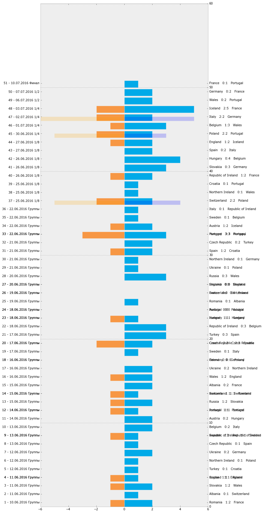

Let's now find out which team scored the most goals. To do this, create a grouped DataFrame from the existing one and calculate some aggregated indicators.

 GAMES_GR = GAMES_F.groupby(['t1']) GAMES_AGG = GAMES_GR.agg({'t1g': np.sum}) GAMES_AGG.sort(['t1g'], ascending=False).head()

teams goals
France 13
Wales 10
Portugal 10
Belgium 9
Iceland 8

Interesting, but let's calculate some more indicators:

Number of matches played
Number of wins / draws / losses
Number of goals scored
Number of matches with extra time
Number of matches, a series of penalties

 GAMES_F['n'] = 1 GAMES_GR = GAMES_F.groupby(['t1']) GAMES_AGG = GAMES_GR.agg({'n': np.sum, 'draw': np.sum, 't1w': np.sum, 't2w':np.sum, 't1g': np.sum, 't2g': np.sum}) GAMES_AGG['games_extra'] = GAMES_GR.apply(lambda x: x[x['t1ge']>0]['n'].count()) GAMES_AGG['games_penalty'] = GAMES_GR.apply(lambda x: x[x['t1gp']>0]['n'].count()) GAMES_AGG.reset_index(inplace=True) GAMES_AGG.columns = ['team', 'draw', 'goals_lose', 'lose', 'win', 'goals', 'games', 'games_extra', 'games_penalty'] GAMES_AGG = GAMES_AGG.reindex(columns = ['team', 'games', 'games_extra', 'games_penalty', 'win', 'lose', 'draw', 'goals', 'goals_lose'])

Now visualize these distributions:

 GAMES_P = GAMES_AGG GAMES_P.sort(['goals'], ascending=False, inplace=True) GAMES_P.reset_index(inplace=True) bar_width = 0.6 fig, ax = plt.subplots(figsize=[16, 6]) ax.bar(GAMES_P.index + 0.2, GAMES_P.goals, bar_width, color='#01aae8', label='') ax.bar(GAMES_P.index + 0.2, -GAMES_P.goals_lose, bar_width, color='#f79744', label='') ax.set_xticks(GAMES_P.index) ax.set_xticklabels(GAMES_P.team, rotation=45) ax.set_ylabel('') ax.set_xlabel('') ax.set_title('   -  ') ax.legend() plt.grid(False) plt.show() fig.savefig(os.path.join(DIR, 'output', 'bar_1.svg'))

At the output we get the following schedule:

The distribution of scored / missed balls Euro 2016 (Python)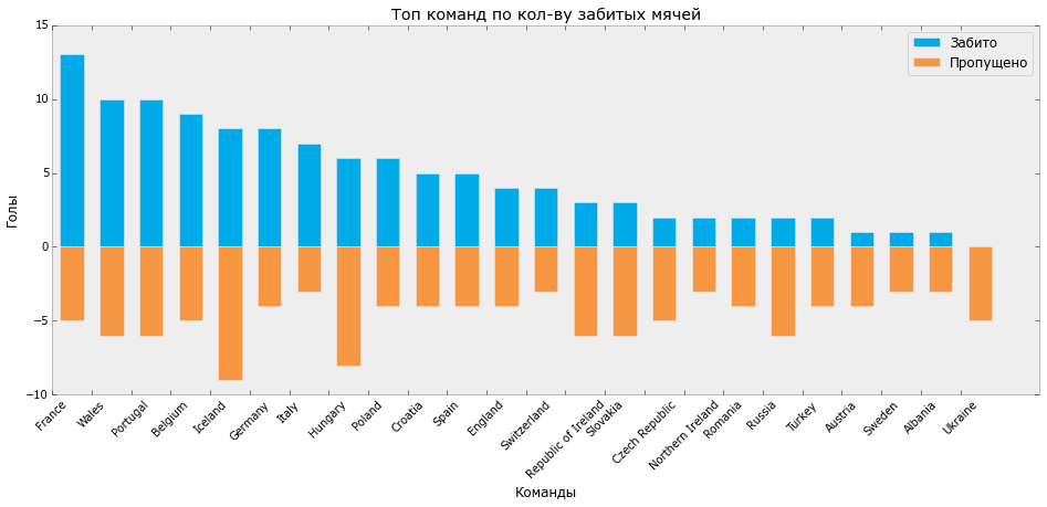

Let's draw another graph of the distribution of victories, defeats and draws on the Euro.

 GAMES_P = GAMES_AGG GAMES_P.sort(['win'], ascending=False, inplace=True) GAMES_P.reset_index(inplace=True) bar_width = 0.6 fig, ax = plt.subplots(figsize=[16, 6]) ax.bar(GAMES_P.index + 0.2, GAMES_P.win, bar_width, color='#01aae8', label='') ax.bar(GAMES_P.index + 0.2, -GAMES_P.lose, bar_width/2, color='#f79744', label='') ax.bar(GAMES_P.index + 0.5, -GAMES_P.draw, bar_width/2, color='#99b286', label='') ax.set_xticks(GAMES_P.index) ax.set_xticklabels(GAMES_P.team, rotation=45) ax.set_ylabel('') ax.set_xlabel('') ax.set_title('   - ') ax.set_ylim(-GAMES_P.lose.max()*1.2, GAMES_P.win.max()*1.2) ax.legend(ncol=3) plt.grid(False) plt.show() fig.savefig(os.path.join(DIR, 'output', 'bar_2.svg'))

At the output we get the following schedule:

Distribution of victories / draws / losses of Euro 2016 (Python)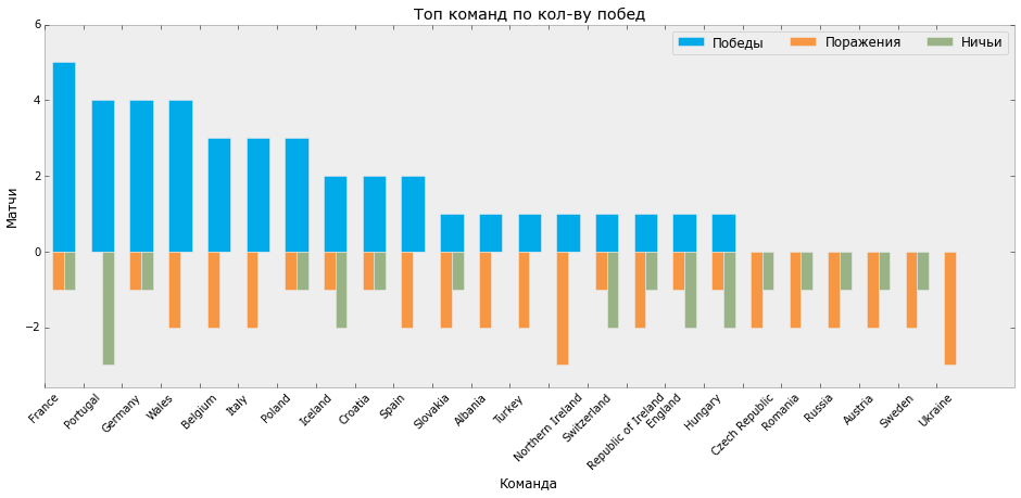

Taking this opportunity, I would like to note that the leader in the number of goals scored and the number of victories France did not win the championship, and Portugal, with 3 matches in a draw, fewer goals scored and more than the number of goals conceded from France, won the cup.

3. Editing vector graphics in Inkscape

Now let's edit the graphics we got in Inkscape vector editor. The choice fell on this editor for one reason - it is free. Immediately I would like to note that it is also extremely demanding of system resources - empirically it was definitely that the minimum amount of RAM for work is 8GB. I had 4GB, so by the end of the editing of one of the illustrations I was already beginning to get nervous about the long wait. For comfortable work in the editor, it is recommended to familiarize yourself with the introductory tutorials on the site.

The main task of editing graphs in the vector editor is the ability to make beautiful visualizations using the built-in functions of the editor. In this case, we can:

Select, modify, and move any graph element created using python
Arrange to add drawn data from external sources, for example, to insert flags of countries
Export data in any resolution to most graphic formats.

I will not long describe the transformations that I did in Inkscape, but simply list them and present the resulting graphs. Changes:

Edited signatures on axes
Removed extra fills
Added country flags for better visualization.
Produced color highlights
Added symbols of Euro 2016
Added football attributes (for example, balls that reflect the number of goals scored on the timeline)

Here's what happened in the end:

Distribution of goals scored / missed balls Euro 2016 (Inkscape)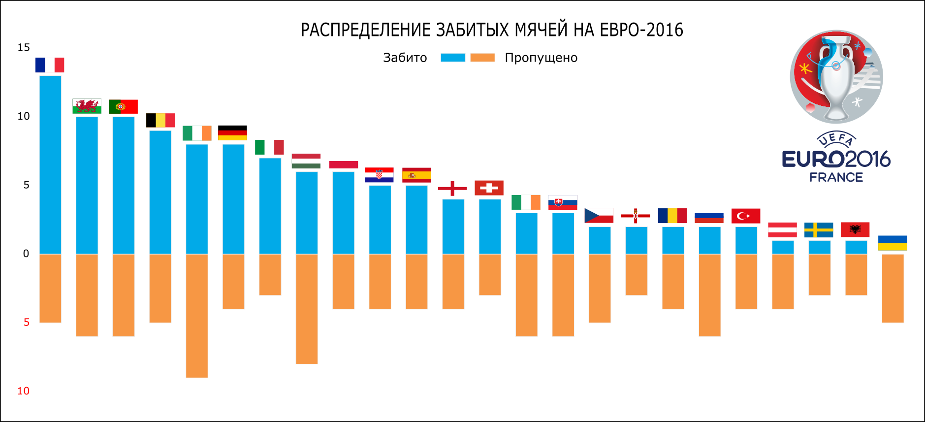

The distribution of wins / losses / draws Euro 2016 (Inkscape)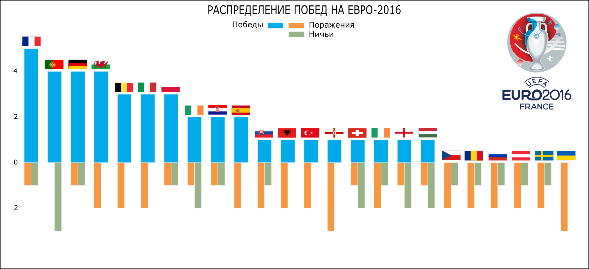

All matches Euro 2016 (Inkscape)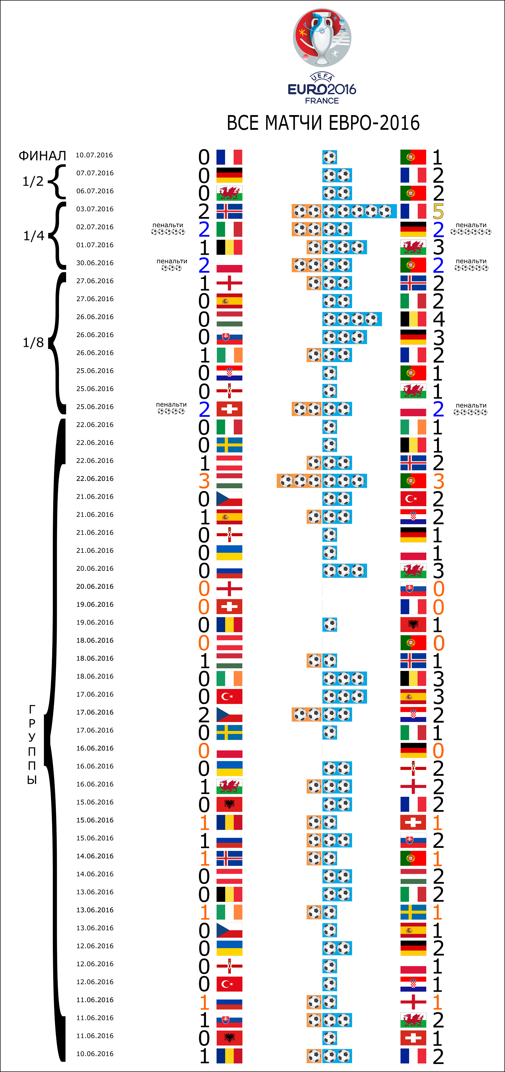

Thanks for attention.

Source: https://habr.com/ru/post/305986/

All Articles

Visualization of Euro 2016 statistics using Python and Inkscape

Content

1. Work with API data

2. Data Visualization with Python

3. Editing vector graphics in Inkscape

More articles: