The TensorFlow project is bigger than you might think. The fact that this is a library for deep learning, and its connection with Google helped the TensorFlow project to attract a lot of attention. But if you forget about the hype, some of its unique details deserve a deeper study:

• The main library is suitable for a wide family of machine learning technicians, and not just for deep learning.
• Linear algebra and other entrails are clearly visible from the outside.
• In addition to the basic machine learning functionality, TensorFlow also includes its own logging system, its own interactive logging visualizer, and even a powerful data delivery architecture.
• The execution model of TensorFlow is different from the scikit-learn of the Python language and most of the tools in R.

All this is cool, but TensorFlow can be quite difficult to understand, especially for someone who is just introduced to machine learning.

How does TensorFlow work? Let's try to figure out, see and understand how each part works. We will examine the data movement graph , which defines the calculations that your data will go through, understand how to train models with a gradient descent using TensorFlow, and how TensorBoard visualizes work with TensorFlow. Our examples will not help solve real-world industrial-level machine learning problems, but they will help you understand the components that underlie everything TensorFlow has created, including what you write in the future!

Names and execution in Python and TensorFlow

The way TensorFlow manages computations is not much different from how Python normally does. In both cases, it is important to remember that, paraphrasing Hadley Wickham , the object has no name (see image 1). To understand the similarities and differences between the principles of Python and TensorFlow, let's take a look at how they refer to objects and handle the calculation.

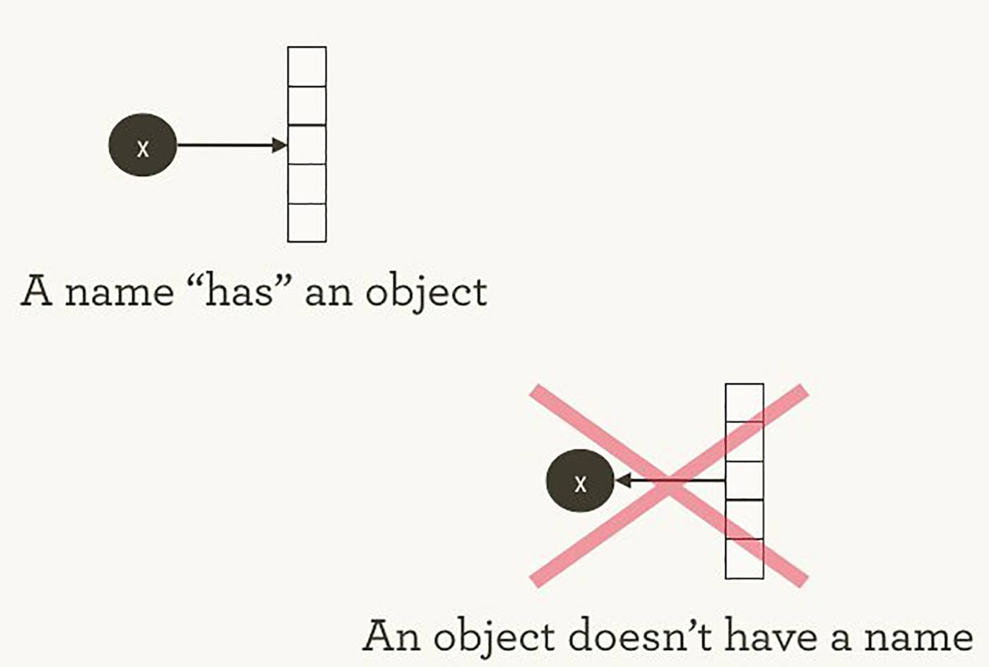
Image 1. The names "have" objects, but not vice versa. Illustration by Hadley Wickham, used with permission.

Variable names in Python are not what they represent. They simply point to objects. So, when you write in Python foo = [] and bar = foo , this does not mean that foo is equal to bar ; foo is bar , in the sense that they both point to the same list object.

 >>> foo = [] >>> bar = foo >>> foo == bar ## True >>> foo is bar ## True 

You can also make sure that id(foo) and id(bar) same. This identity, especially with variable data structures like lists, can lead to serious bugs, if you misunderstand it.

Inside Python, it manages all your objects and keeps track of the names of the variables and which object each name refers to. The TensorFlow graph represents another layer of this type of control. As we will see later, names in Python will refer to objects that are connected to more detailed and more clearly controlled operations on the TensorFlow graph.

When you enter a Python expression, for example, in the interactive interpreter REPL (Read Evaluate Print Loop), everything you type will almost always be calculated right away. Python is eager to do what you order. So if I tell him to do foo.append(bar) , he will immediately add, even if I never use foo .

A more lazy alternative is just to remember what I said to foo.append(bar) , and if at some point in the future I’ll compute foo , then Python will add. This is closer to how TensorFlow behaves: in it the definition of a relationship has nothing to do with the calculation of the result.

TensorFlow separates the definition of computation from its execution even more strongly, since they occur generally in different places: the graph defines operations, but operations occur only within sessions. Graphs and sessions are created independently of each other. A graph is something like a drawing, and a session is something like a construction site.

Returning to our simple Python example, let me remind you that foo and bar point to the same list. Adding bar to foo , we inserted the list inside. You can imagine this as a graph with a single node that points to itself. Nested lists are one of the ways to represent the structure of a graph, similar to the computational graph TensorFlow.

 >>> foo.append(bar) >>> foo ## [[...]] 

Real TensorFlow graphs will be more interesting!

Simplest graph TensorFlow

To immerse yourself in the topic, let's create a simplest TensorFlow graph from scratch. Fortunately, TensorFlow is easier to install than some other frameworks. The example here will work with Python 2.7 or 3.3+, and we are using TensorFlow 0.8.

 >>> import tensorflow as tf 

By this time, TensorFlow has already started managing a bunch of fortunes for us. For example, an explicit default column already exists. Inside the default graph is in _default_graph_stack , but we do not have access there directly. We use tf.get_default_graph() .

 >>> graph = tf.get_default_graph() 

The nodes of the TensorFlow graph are called operations (“operations” or “ops”). A set of operations can be seen using graph.get_operations() .

 >>> graph.get_operations() ## [] 

Now in the graph is empty. We will need to add there everything that the TensorFlow library will need to calculate. Let's start by adding a simple constant with a value of one.

 >>> input_value = tf.constant(1.0) 

Now this constant exists as a node, an operation in the graph. The Python name of the variable input_value indirectly refers to this operation, but it can also be found in the default column.

 >>> operations = graph.get_operations() >>> operations ## [<tensorflow.python.framework.ops.Operation at 0x1185005d0>] >>> operations[0].node_def ## name: "Const" ## op: "Const" ## attr { ## key: "dtype" ## value { ## type: DT_FLOAT ## } ## } ## attr { ## key: "value" ## value { ## tensor { ## dtype: DT_FLOAT ## tensor_shape { ## } ## float_val: 1.0 ## } ## } ## } 

TensorFlow uses the protocol buffers format inside. ( Protocol buffers are something like Google-level JSON ). Displaying the node_def the constant operation above shows that TensorFlow stores in the protocol buffer view for the number one.

People who are not familiar with TensorFlow sometimes wonder what the essence of creating "TensorFlow-versions" of existing things is. Why not just use a regular Python variable instead of further defining a TensorFlow object? One of the TensorFlow tutorials has an explanation:

To make effective numerical computations in Python, libraries like NumPy are usually used, which perform such expensive operations as matrix multiplication outside of Python using highly efficient code implemented in another language. Unfortunately, there is an additional load when switching back to Python after each operation. This load is especially noticeable when you need to perform calculations on a GPU or in distributed mode, where data transfer is an expensive operation.

TensorFlow also does complex computations outside of Python, but it goes even further to avoid additional workload. Instead of running a single expensive operation independently of Python, TensorFlow allows us to describe a graph of interacting operations that work completely outside of Python. A similar approach is used in Theano and Torch.

TensorFlow can do a lot of cool stuff, but it can only work with what has been explicitly transferred to it. This is true even for one constant.

If you look at our input_value , you can see it as a 32-bit zero-dimensional tensor: just one number.

 >>> input_value ## <tf.Tensor 'Const:0' shape=() dtype=float32> 

Note that the value is not specified . To calculate input_value and get a numerical value, you need to create a "session" in which you can calculate the operations of the graph, and then explicitly calculate or "run" input_value . (Session uses default graph).

 >>> sess = tf.Session() >>> sess.run(input_value) ## 1.0 

It may seem strange to "run" a constant. But this is not much different from the usual Python expression evaluation. TensorFlow simply manages its own data space - a computational graph, and it has its own methods for computing.

The simplest neuron TensorFlow

Now that we have a session with a simple graph, let's build a neuron with one parameter or weight. Often, even simple neurons also include the bias term and non-identity activation function, but we can do without them.

The weight of the neuron will not be constant. We expect it to change when learning, based on the truth of the input and output used for training. Weight will be variable TensorFlow. We give it an initial value of 0.8.

 >>> weight = tf.Variable(0.8) 

You might think that adding a variable will add an operation to the graph, but in fact this line alone will add four operations. You can find out their names:

 >>> for op in graph.get_operations(): print(op.name) ## Const ## Variable/initial_value ## Variable ## Variable/Assign ## Variable/read 

You don’t want to analyze each operation “for the bones” for too long, let's better create at least one similar to the present calculation:

 >>> output_value = weight * input_value 

Now there are six operations in the graph, and the last one is multiplication.

 >>> op = graph.get_operations()[-1] >>> op.name ## 'mul' >>> for op_input in op.inputs: print(op_input) ## Tensor("Variable/read:0", shape=(), dtype=float32) ## Tensor("Const:0", shape=(), dtype=float32) 

Here you can see how the multiplication operation monitors the source of input data: they come from other operations in the graph. It is quite difficult for a person to keep track of all the connections in order to understand the structure of the entire graph. The visualization of the TensorBoard graph is designed specifically for this.

How to determine the result of multiplication? It is necessary to "start" the operation output_value . But this operation depends on the variable weight . We indicated that the initial weight value should be 0.8, but the value has not yet been set in the current session. The tf.initialize_all_variables() function generates an operation that initializes all variables (in our case only one), and then we can start this operation.

 >>> init = tf.initialize_all_variables() >>> sess.run(init) 

The tf.initialize_all_variables() includes initializers for all variables that are currently in the graph , so if you add new variables, you will need to run tf.initialize_all_variables() again; simple init will not include new variables.

Now we are ready to start the operation output_value .

 >>> sess.run(output_value) ## 0.80000001 

This is 0.8 * 1.0 with 32-bit floats, and 32-bit floats barely understand the number 0.8. A value of 0.80000001 is the closest thing they could do.

We look at the graph in TensorBoard

Our graph is still quite simple, but it would already be nice to see its presentation in the form of a diagram. Use TensorBoard to generate such a chart. TensorBoard reads the name field that is stored in each operation (this is not at all the same as Python variable names). You can use these TensorFlow names and switch to more familiar Python variable names. Using tf.mul equivalent to simply multiplying with * in the example above, but here you can set a name for the operation.

 >>> x = tf.constant(1.0, name='input') >>> w = tf.Variable(0.8, name='weight') >>> y = tf.mul(w, x, name='output') 

TensorBoard looks into the output directory created from TensorFlow sessions. We can write to this output using SummaryWriter , and if we do nothing except one graph, only one graph will be recorded.

The first argument to create a SummaryWriter is the name of the output directory that will be created if necessary.

 >>> summary_writer = tf.train.SummaryWriter('log_simple_graph', sess.graph) 

Now you can run TensorBoard on the command line.

 $ tensorboard --logdir=log_simple_graph 

TensorBoard runs as a local web application on port 6006. (“6006” is “goog” upside down). If you go to the browser on localhost:6006/#graphs , then you can see the graph of the graph created in TensorFlow. It looks something like image 2.

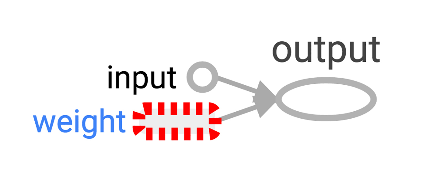
Image 2. TensorBoard visualization of the simplest TensorFlow neuron.

We learn neuron

We created a neuron, but how will it learn? We set the input value to 1.0. Suppose the correct final value is zero. That is, we have a very simple data set for learning with one example with one characteristic: the value is one and the mark is zero. We want to teach a neuron to convert one to zero.

Now the system takes a unit and returns 0.8, which is not the correct behavior. We need a way to determine how wrong the system is. We call this measure of erroneousness “loss” (“loss”) and set the goal of the system to minimize the loss. If the loss can be a negative number, then minimization does not make sense, so let's define the loss as the square of the difference between the current input value and the desired output value.

 >>> y_ = tf.constant(0.0) >>> loss = (y - y_)**2 

Up to this point, nothing in the graph is learning. For training, we need an optimizer. We use the gradient descent function to be able to update the weight based on the value of the derivative loss. The optimizer needs to set the training level to control dimensional updates, we will set 0.025.

 >>> optim = tf.train.GradientDescentOptimizer(learning_rate=0.025) 

The optimizer is unusually smart. It can automatically detect and use the desired gradient at the level of the entire network, making a step-by-step backward movement for learning.

Take a look at what the gradient looks like for our simple example.

 >>> grads_and_vars = optim.compute_gradients(loss) >>> sess.run(tf.initialize_all_variables()) >>> sess.run(grads_and_vars[1][0]) ## 1.6 

Why the gradient value is 1.6? The loss value is squared, and the derivative is an error multiplied by two. Now the system returns 0.8 instead of 0, so the error is 0.8, and the error multiplied by two is 1.6. Works!

In more complex systems, it will be especially useful that TensorFlow automatically calculates and applies these gradients for us.

Let's apply a gradient to end back propagation.

 >>> sess.run(optim.apply_gradients(grads_and_vars)) >>> sess.run(w) ## 0.75999999 # about 0.76 

The weight decreased by 0.04 because the optimizer took away the gradient multiplied by the learning level, 1.6 * 0.025, moving the weight in the right direction.

Instead of leading the optimizer by the handle in this way, you can do an operation that calculates and applies the gradient: train_step .

 >>> train_step = tf.train.GradientDescentOptimizer(0.025).minimize(loss) >>> for i in range(100): >>> sess.run(train_step) >>> >>> sess.run(y) ## 0.0044996012 

After launching the training step several times, the weight and final value became very close to zero. Neuron learned!

Diagnostics training in TensorBoard

We may be wondering what happens during training. For example, we want to follow up on what the system predicts at every step of the training. You can display the value on the screen at each step of the cycle.

 >>> for i in range(100): >>> print('before step {}, y is {}'.format(i, sess.run(y))) >>> sess.run(train_step) >>> ## before step 0, y is 0.800000011921 ## before step 1, y is 0.759999990463 ## ... ## before step 98, y is 0.00524811353534 ## before step 99, y is 0.00498570781201 

It will work, but there are some problems. Difficult to perceive the list of numbers. The schedule would be better. Even with one output value too much. And we probably want to follow a few values. It would be nice to write more systematically.

Fortunately, the same system that was used to visualize the graph includes the mechanism we need.

Add to the computation graph an operation that briefly describes its state. In our case, the operation reports the current value of y , the current output of the neuron.

 >>> summary_y = tf.scalar_summary('output', y) 

Running this operation returns a string in the protocol buffer format that can be written to the logs directory using the SummaryWriter .

 >>> summary_writer = tf.train.SummaryWriter('log_simple_stats') >>> sess.run(tf.initialize_all_variables()) >>> for i in range(100): >>> summary_str = sess.run(summary_y) >>> summary_writer.add_summary(summary_str, i) >>> sess.run(train_step) >>> 

Now, after running tensorboard --logdir=log_simple_stats , an interactive graph is displayed on the localhost:6006/#events page (Figure 3).

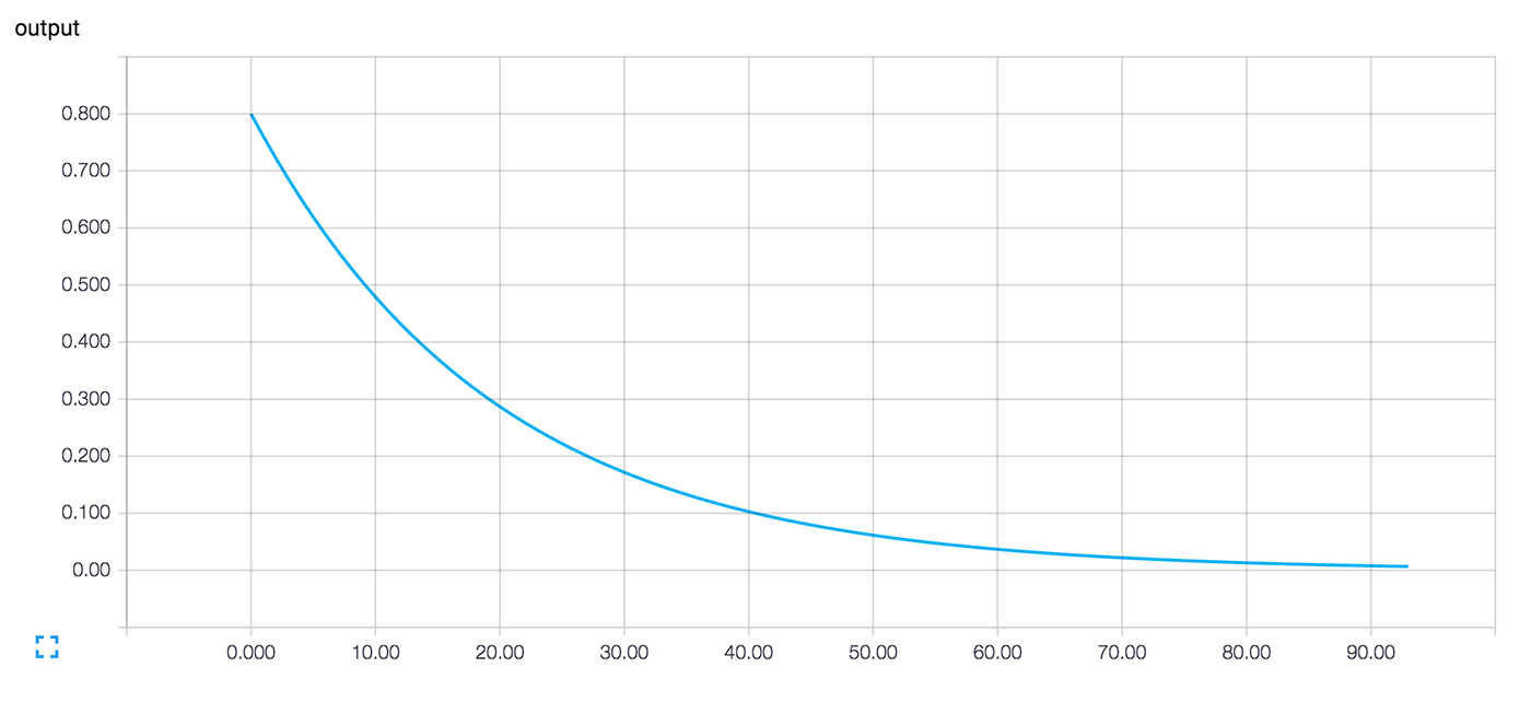
Image 3. TensorBoard visualization of the output value of the neuron and the number of training iteration.

Moving on

Here is the final version of the code. There is not much of it, and each part shows the useful (and understandable) functionality of TensorFlow.

 import tensorflow as tf x = tf.constant(1.0, name='input') w = tf.Variable(0.8, name='weight') y = tf.mul(w, x, name='output') y_ = tf.constant(0.0, name='correct_value') loss = tf.pow(y - y_, 2, name='loss') train_step = tf.train.GradientDescentOptimizer(0.025).minimize(loss) for value in [x, w, y, y_, loss]: tf.scalar_summary(value.op.name, value) summaries = tf.merge_all_summaries() sess = tf.Session() summary_writer = tf.train.SummaryWriter('log_simple_stats', sess.graph) sess.run(tf.initialize_all_variables()) for i in range(100): summary_writer.add_summary(sess.run(summaries), i) sess.run(train_step) 

This example is even simpler than the examples from Neural Networks and Deep Learning by Michael Nielsen, which served as inspiration. Personally, the study of such details helps me to understand and build more complex systems that use simple building blocks as a basis.

If you want to continue experiments with TensorFlow, then I advise you to try to make more interesting neurons, for example, with a different activation function . You can make training with more interesting data. You can add more neurons. You can add more layers. You can dive into more complex ready-made models , or spend more time studying your own manuals and TensorFlow guides. Successes!