Machine learning instead of DPI. Building a traffic classifier

One can hardly imagine the world of modern network technologies without DPI (deep packet inspection). It contains the systems for detecting network attacks, the lion's share of corporate network security policies, shaping and blocking user traffic by the telecom operator - yes, each provider must have a DPI tool to fulfill the requirements of Roskomnadzor.

And yet, with all its relevance, DPI has some drawbacks. The main one is that the DPI tools need to see the payload of the analyzed packets. And what to do when the client uses encryption? Or, for example, if we do not have DPI here and now, but in the future we will need to carry out some analysis of the current traffic on the network - then we just have to save all the payload for subsequent analysis, which is very inconvenient.
')
In this article, I want to propose an alternative way to solve one of the main tasks of the DPI — to determine the application-level protocol — based on a very small amount of information, without checking the list of well-known ports and not looking at the packet payload. At all.

Solution approach

First, let's decide on the object of classification - for which entity will we define the application layer protocol?

In DPI means, as a rule, the object of classification is the traffic flow of the transport layer - this is a set of IP packets that have the transport layer protocol and an unordered pair of endpoints: <(source ip, source port), (destination ip, port destination)>. We will also work with such flows.

The idea behind the proposed method is that different applications using different protocols also generate transport layer flows with different statistical characteristics. If we accurately and concisely determine the set of statistical flow metrics, then using the values ​​of these metrics it will be possible to predict with high accuracy which application generated this flow and, accordingly, which application layer protocol is transferred by this flow.

Before defining these metrics, we introduce a couple of definitions:

• Client - initiator of TCP connection or sender of the first UDP datagram of the stream, depending on the transport layer protocol;
• The server is the receiving side of the TCP connection or the destination of the first UDP datagram of the stream, depending on the transport layer protocol.
• A chunk of data is a collection of application-level payloads that were transferred from one side to the other (from the client to the server or vice versa) and were not interrupted by the payload from the other side.

The latter definition requires some explanation, so my inner Michelangelo to the rescue:


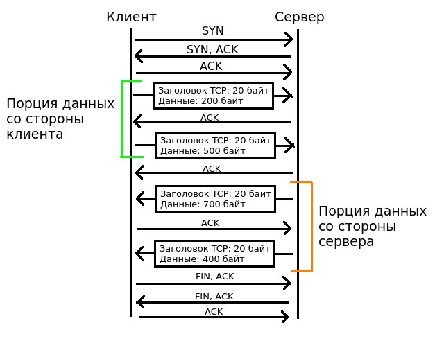
In this example, after the TCP handshake, the client begins to transmit the payload — hence, a portion of the data from the client begins. While the server does not send any payload in response, but merely sends an ACK, a portion of the data from the client continues. When the server feels the need to transfer some load of the application layer, the portion of the client data ends and the portion of the server data begins. As it is easy to understand, the entire transfer of the payload is an alternation of chunks of data from one side to the other. With a very intensive exchange of data from both sides of the data can degenerate into separate IP packets.

Statistical flow metrics

All of our statistical flow characteristics will dance around four rows of numbers:

• The sequence of sizes of transport layer segments (TCP or UDP) sent from the client;
• The sequence of sizes of the transport level segments sent from the server side;
• The sequence of the sizes of the chunks of data sent by the client;
• The sequence of the sizes of the chunks of data sent by the server;

For the short example shown in the figure above, this series will have the following meanings:

• Client side segment sizes: [220, 520]
• Server-side segment sizes: [720, 420]
• Client data sizes: [700]
• The size of the chunks of data from the server: [1100]

These 4 rows of numbers (as we will see later) very well characterize the data flow, and based on them you can quite accurately guess the application layer protocol.

Turning on the fantasy, we formulate the statistical characteristics of the data stream, starting from these 4 rows of numbers:

1. Client-side average packet size
2. Standard deviation of packet size on the client side
3. Server-side average packet size
4. Standard server packet size deviation
5. Average client data size
6. Standard deviation of the portion of data from the client
7. Average server chunk size
8. Standard deviation of the data portion size on the server side
9. Average number of packets per client data portion
10. Average number of packets per server data portion
11. Client's efficiency - the amount of application load transferred, divided by the total amount of application and transport load transferred
12. Server efficiency
13. Ratio of bytes - how many times the client transmitted more bytes than the server
14. Payload Ratio - how many times the client transmitted more bytes than the server
15. Package Ratio - how many times the client has transmitted more packets than the server
16. The total number of bytes transferred by the client
17. The total amount of application load transferred from the client
18. The total number of transferred segments of the transport layer from the client
19. The total number of transferred pieces of data from the client
20. Total number of bytes transferred by the server
21. The total amount of application traffic transferred from the server side
22. The total number of transmitted segments of the transport layer from the server
23. The total amount of data transferred by the server
24. The size of the first segment of the transport level from the client
25. Client’s second transport segment size
26. The size of the first segment of the transport layer on the server side
27. The size of the second segment of the transport layer on the server side
28. The size of the first portion of data from the client
29. The size of the second portion of data from the client
30. The size of the first portion of data from the server
31. The size of the second portion of data from the server
32. Protocol type of the transport layer (0 - UDP, 1 - TCP)

Now we need to clarify a few points.

First, the signs of the “total X” type are unstable in themselves, because their value depends on how long we observe the flow. The more we observe, naturally, the more bytes will be transferred, and the application load, and segments, and chunks of data. In order to add certainty to these indicators, in the future we will not consider the entire stream from the beginning of the observation to the end, but a certain section of each stream along the first N segments of the transport layer. When calculating all the listed metrics, we will use only the first N segments.

Secondly, it may not be clear why we need in terms of the size of the first and second segments and portions of data from each side. As shown in one of the scientific papers on this topic ^[1] (link in the sources), the size of the first few IP packets can carry a lot of information about the protocol used. So these indicators will not be superfluous.

Now we will define how we will try to guess the application-level protocol of a specific flow, having the calculated statistical metrics on hand. Machine learning will help us here. The task in question is in its classical formulation the task of classifying objects into several classes.

Each object has as many as 32 characteristics, and the relevance of each of them to an object’s class label at this stage of the study remains in question. Therefore, it would be wise to choose the popular machine learning algorithm, Random Forest, because it is not very sensitive to noise and feature correlation (and some of our statistical metrics are likely to correlate strongly with each other).

This algorithm works on the principle of "learning with the teacher." This means that we need some sample of objects for which class labels are already known. We will divide this sample in the ratio of 1 to 2 for training and testing. We will train the model on the training set (in our case, the training consists in building a set of decision trees), and on the test set we will evaluate how well the model copes with the task.

Harvest time

With the methodology of the experiment, now everything is clear, it remains to find the traffic itself, the characteristics of which we will calculate.

No provider, of course, will allow us to collect traffic into its network - who knows there, what data will we collect? We will manage artisanal conditions. For several days I spent capturing the traffic of my own computer, doing normal business along the way - I sat in VK, watched a video on Youtube, made some calls on Skype, downloaded a couple of torrents. The result was more than 3 GB of captured traffic.

Now, remember that in addition to the traffic itself, we also need for each captured stream to reliably determine the application layer protocol that it transfers. And this is where the DPI tools will help us, specifically the nDPI library. Included with this library is an example of a traffic analyzer called ndpiReader, which will be useful to us. A nice bonus is that this application will separate all of our raw traffic dumps into traffic flows for us, so we don’t even have to do this.

But still it will be necessary to delve into the depths of pcap files. For this we use the dpkt library. Unfortunately, it was not ported to the third version of Python, so the script for processing pcap files will be written in the second version of the language.

Putting it all together, we’ll write a script that converts PCAP files to a feature table and exports it to CSV format. Link to the repository with this script at the end of the article.

What time is it? Classification time!

Yes, yes, we finally got to what it was all about!

But before pushing the entire table of attributes from the ship to the ball into the first Random Forest, consider the data a little more closely. Here is a list of application protocols and the number of streams of each protocol that is in our sample:



The first thing I want to do is merge all SSL_No_Cert traffic into SSL, because this is essentially the same thing.

The second is kicking traffic from Apple, NTP, Unencrypted_Jabber and Unknown. The first three protocols have too few streams to classify, and under Unknown anything can be hidden.

Now we divide our data into training and test samples. We get this:



After several experiments, the following values ​​were chosen as parameters of the Random Forest algorithm:

• Number of trees: 27
• Criterion: entropy
• Maximum tree depth: 9

Recall that some of our statistical characteristics oblige us to fix the volume of traffic under consideration for each stream. To begin, take a more traffic cutoff - the first 1000 segments in each stream. Let us check whether the application-level protocol can be predicted by our statistical metrics at all. Drumroll!



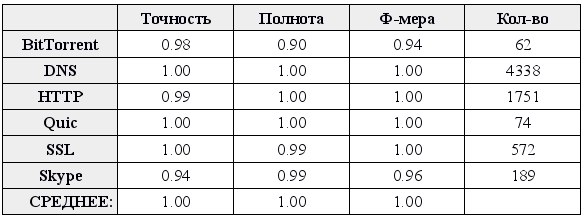
Above is a table of the accuracy and completeness of the predictions for each class. Accuracy for class K is the proportion of predictions of the form “object X belongs to class K”, which turned out to be correct. Completeness for class K - the number of objects X, which are recognized by the classifier as belonging to the class K, divided by the total number of objects belonging to the class K. F-measure is the harmonic mean of completeness and accuracy.

Well, a little more simple table:



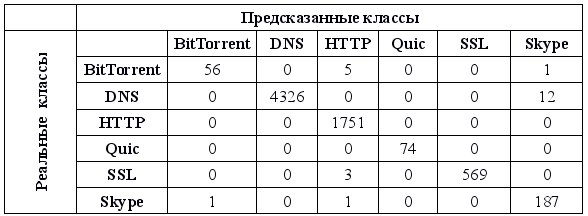
Here, in each cell, a number is indicated, which means the number of cases when the traffic flow belonging to the class specified in the row header was classified as belonging to the class specified in the column header. That is, the numbers on the main diagonal are correct classifications, the numbers outside it are all sorts of errors.

In general, it seems that the classifier does its job well. With the exception of rare errors, all predictions are correct.

The Random Forest machine learning algorithm is also good in that it can give us information about which signs turned out to be more useful than others. Out of curiosity, take a look at the most important signs:



Top stably occupy the signs, tied to the statistical characteristics of the client side. From this we can conclude that it is the customers of different applications that differ the most, and the servers - less.

From the server, only the size of the second packet got lost. This is easily explained by the fact that by the size of the second packet, you can easily select SSL from the rest of the traffic, because in the second packet of the server a certificate is transmitted.

It is pleasantly surprising that the protocol type of the transport level is included only in the TOP-10 of the most important signs - although it would seem that a lot of information is contained in this attribute! So, in our statistical metrics information is much more.

I also want to note that when the semen of the pseudo-random number generator changes, the top of the most important signs changes somewhat. What remains common is that customer-related metrics are consistently above, but their order is changing. A protocol transport level jumps between the first and tenth place.

Now the fun part. Before that, we took a slice of the first 1000 segments of each stream, and based on this slice we calculated statistical metrics. A natural question arises: how much can this slice be reduced and still get good classification indicators?

The answer is discouraging. You can omit the number of segments in each stream to ... three. Not including TCP handshake, of course, because it does not carry any information.

Below are the values ​​of completeness and accuracy for each class, a table of real and predicted classes and top characteristics when building and testing a model on only the first three segments of the transport layer (for TCP, these are actually 6 segments, the first three are discarded).







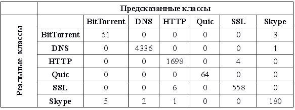
The attentive reader may notice that the total number of records in the sample has become less compared to the previous case. The fact is that for the calculation of most characteristics it is necessary that there should be at least one piece of data from the client and at least one from the server. If it turns out that in the first 3 segments only the client or only the server transmitted, such a stream is rejected at the stage of drawing up the table of attributes.

The result was unexpected because with a sharp decrease in the number of segments in each stream, the quality of the classification did not deteriorate, but even somewhat improved. This can be attributed to the fact that it is the first segments transferred that carry the greatest information about the type of application. Therefore, as the number of segments decreases, our statistical metrics begin to carry information only about the first segments, but not about all, and the quality of the classification slightly increases.

Conclusion

In this article, I clearly demonstrated how to perform a sufficiently high-quality traffic analysis in order to determine the application-level protocol without DPI tools. That is characteristic, it is possible to determine the application protocol with sufficient accuracy by the first several transmitted segments of the transport layer.

All developed code is posted in the repository on github . The readme repository gives instructions on how you can repeat the results obtained in the article. The csv folder contains the attribute tables obtained after processing the collected PCAP files. But you will not find PCAP files there - I apologize, but the confidentiality of my data is above all.

As a visual illustration of the real-time classifier operation, I developed a simple application on PyQt4 . And even recorded a video with a demonstration of his work .

For what can be applied the stated approach? For example, to identify the application layer protocols used in those conditions when the payload is encrypted (hello, paranoia). Or, for the proactive collection of statistics for analysis in case such an analysis is required - after all, to determine the application layer protocol, it is enough to have only 256 bytes of information per stream (32 floating point numbers).

Thanks

I want to thank Daniel Prokhorov and Nadezhda Troflyanina, with whom we were engaged in the development of this idea, collected traffic and then spoke at the VII Youth Scientific Forum of MTUCI.

Sources

It would be wrong not to specify the scientific work, from which we drew inspiration and some good ideas:

1. Internet Traffic Classification Demystified: On the Sources of the Discriminative Power
2. SVM Based Network Traffic Classification Using Correlation Information
3. Internet Traffic Classification Using Bayesian Analysis Techniques