Prediction of the likelihood of each client’s transition to the status of a former member

The authors of the publication are Dmitry Sergeev and Julia Petropavlovskaya .

The first in Russia Virtual hackathon from Microsoft, with the support of Forbes, recently ended. Our two-person team managed to win first place in the WorldClass nomination, which required predicting the likelihood of each client’s transition to the status of a former club member. In this article we would like to share our decision and talk about its main stages.


')

Data preparation

Most of the time was spent in cleaning, restoring and combining data, since datasets were heavily polluted and grouped into four separate categories:

• Customer contracts
• Attendance
• Frost
• Communication between customers and the club

Test and training data sets were broken down by months. Train contained customer information for December 2015, and Test - for March 2016. For each of the categories, we combined the Train and Test parts for further processing.

Customer contracts

Contracts were the first data set we took on, since it was there that the target variable was contained - “did the client extend his contract”, as well as the contract codes and clients in the amount of 17,631 pieces that served as keys for merging all the other datasets. A small number of missing values ​​in the variables were restored by the mods. Then they created features for the season (winter, spring ...), the month and the day on which the contract was signed with the club, and the variables "contract duration", "rest of freezing days" and "balance of bonuses in the account". Various categorical variables, such as age group, club segment, etc. left unchanged.

Attendance

We started by creating a variable - the duration of a one-time hike to the fitness club.



It turned out that particularly diligent customers can spend almost 9 hours on the club’s territory, possibly due to the passage of complex procedures.

Also in dataset there were categorical variables, the gradations of which we decided to group into more general categories. For example, "Category Manager":

additional = [' ', ''] coach = [' ', " "] coach_vip = [" ", " "] other = [''] 

Similarly, “Service Direction”:

 sport = [" ", " ", "", " ", "Mind Body", " ", " ", "", " "] health_beauty = ["", " ", " ", ", ", "_SF", " ", " ", " ", " ", "", " _SF", "", "_SF", "  ", "", "  SPA", " ", "_SF", "SPA"] 

Finally, they added a variable with the frequency of visits to the club per month and the total number of visits in different seasons (winter, spring ..) and grouped the data by customer codes contained in the contracts by date. Total of 3,700,000 records left ~ 15,000 observations.

Frost

Initially we found out that there are duplicates in dataset. After a little research, it turned out that the same contract number with the same freezing operations is contained in both Train and Test, since the client history of frost was transferred to the test set. In order to avoid retraining models in the future, we threw out duplicate values ​​from the test.

During the year, each client could freeze his card several times, and it seemed to us useful in some form to preserve the temporary structure of its frost. To do this, we created four variables for each season of the year, in which we recorded the total number of freezing days spent in a particular season. As a result, we obtained the following data structure:

Communications

There were three main columns in the raw data: "Date" , "View" and "State" of interaction. Under the "view" hiding such options as "phone call" , "meeting" , "sms" , etc., "state" was characterized by three levels: "took place" , "canceled" , "scheduled" . As in the frosts, we first removed duplicates from the test data in order to clear them from the client history, and then proceeded to create variables.

Almost every client had several dozen communications of one kind or another. To compress this information into a single line for later merging by a unique contract code, we created several new features.

First, we broke the variable "Type of interaction" into 3 dummies:

• personal meeting
• phone
• other

Then they calculated for each client the total and successful ( "held" ) number of communications. By dividing one another, the variable "share of successful communications" was obtained.

The latest finding was the creation of a dummy variable “have there been communications in the past two months”. We assumed that if a person is going to renew his contract, he will try to somehow contact the club when his current contract comes to an end.

As a result, out of 1,500,000 lines, we received 15,500 and combined them with the final dataset. After converting categorical variables to dummy, the number of columns swelled to 72 pieces.

Machine learning

So, the binary classification of clients, classes are approximately equally divided, everything is good and you can learn. In addition to the obvious , the candidates for the model are:

• Random forest
• Neural Network
• SVM
• k-nn
• Naive bayes
• Logit regression
• Decision stumps

Each of the classifiers, in general, showed very good results on validation. Random Forest for 1000 trees with a 10-fold cv gave 0.9499 AUC, a two-layer neural network was able to raise the result to 0.98, and the storm of competition on Kaggle, XGB, showed an impressive 0.982. Also xgboost helped with the visualization of the importance of the signs:



The first three are quite expected - "contract length" , "bonus points balance" and "average visit length" . Also in the first ten are “the number of successful communications” , “the rest of the days of freezing” and, suddenly, “did fitness work in winter” .

The remaining models, except for decisive hemp, on average, gave 0.92–0.94 AUC and were added to the ensemble to reduce the correlation between various predictions.

The ensemble was conceived in the form of two levels - on the first hundred decision stumps, the predictions for which were combined using the majority vote principle, i.e. if 51 stubs were “for” and 49 “against”, then one was put. On the second, the predictions for the other classifiers were connected for later merging.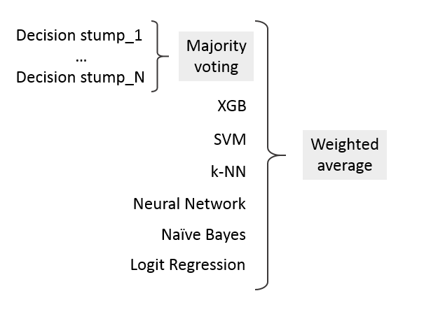



To create an ensemble, the weighted average method was used, each classifier is trained separately, and then a linear combination is created from their predictions:



aj - the weights with which the predictions are included in the ensemble
yj (x) - individual predictions of classifiers
p - the number of models used

Weights were determined by minimizing the ensemble's logloss, with the help of the remarkable function minimize , which returned the optimal values ​​of the weights vector x0.

 from scipy.optimize import minimize opt = minimize(ensemble_logloss, x0=[1, 1, 1, 1, 1, 1, 1]) 

Models that were given a negative weight were thrown out of the ensemble in order to avoid fitting the training data, although there is an interesting opinion that it is not necessary to do this in the case of negatively correlated model errors.

As a result of this selection, the logistic regression disappeared and, unfortunately, all hemp, but the AUC increased by a few thousandth of a percent and amounted to 0.98486. Totally worth it.

Finally, predictions were made on the test dataset, and in order to have at least some idea of ​​their quality, two histograms were built: the first for the client’s predicted extension of the contract for the validation sample, and the second for the test sample.



If we assume that the Train and Test samples were more or less homogeneous, and the number that lasted should be approximately equal to the number of refusals, then there is more than a double overestimation by the models of the probability of contract extension. However, we decided to trust the decision of the ensemble and did not punish him for excessive impudence optimistic forecast. And as it turned out - not in vain.

In conclusion, I would like to thank the organizers of the hackathon for a very interesting practical task and an unforgettable experience.

Link to the repository.