ANOVA, or who comments?

In the comments, the thought was slipping that people did not comment much on articles on Habrahabr, because afraid to lose karma. It turns out that basically those who have more karma write. We will try to investigate this hypothesis in more detail and obtain results supported not only intuitively, but also statistically .
We need to check whether the user's karma has a statistically significant effect on the number of comments that he leaves on average. Since the number of compared groups will be more than two, then the t-test will not work, and it will be necessary to use analysis of variance - this is what ANOVA (analysis of variance) stands for.
I will use the data previously collected by varagian and posted here :
user_data <- read.csv('user_dataset.csv', stringsAsFactors=F, na.strings=c("", "NA")) For single factor analysis of variance, two variables will be needed:
')
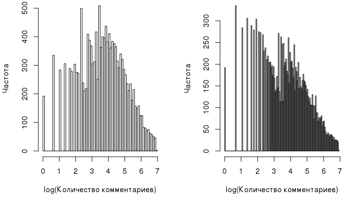
- The dependent variable, which in this case is the number of comments left by the user. Its histogram looks like this:

And such a distribution is not the best for analysis of variance, since for it, certain prerequisites must be fulfilled, such as, for example, the normality of the dependent variable. Fortunately, in this case, the variable can be “made” almost normal by using its log transformation:comments_log <- log1p(user_data$comments)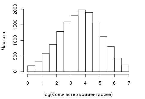
- A factor variable whose effect on the dependent variable is being investigated. Look at the distribution of karma:
summary(user_data$karma) Min. 1st Qu. Median Mean 3rd Qu. Max. 0.00 0.00 5.00 17.92 18.00 1230.00
To group the data, we introduce a new variable, which will be an interval “slice” of karma and play the role of a factor variable:karma_cut <- cut(user_data$karma, breaks=c(-Inf, 0, 5, 15, 25, 50, 100, Inf)) table(karma_cut) (-Inf,0] (0,5] (5,15] (15,25] (25,50] (50,100] (100, Inf] 5488 2059 2955 1423 1411 859 480
The largest group is users with a karma less than or equal to 0.
Nota bene!
Here I must say a few words about the conversion of a continuous variable into a categorical. This practice is widespread in sociological, psychological and biomedical research: for example, the amount of blood pressure can be conditionally defined as low, normal, high. But in general, from a statistical point of view, this procedure is somewhat flawed, since any partitioning is very conditional, potentially leading to loss of information.
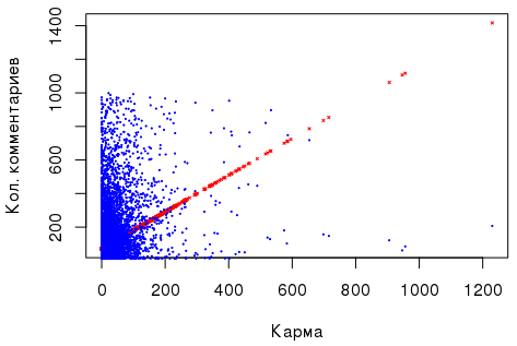
As for the “number of comments” ~ “karma” dependence, there is a slight positive correlation, and the linear regression, performed on the basis of these two numerical indicators (see above), being significant, looks unconvincing, so that statistical findings: for example, Ramsey’s RESET test signals missing variables, and Broish – Pagan’s test indicates heteroskedasticity of random errors. In addition, I set the task in advance to compare groups of users whose karma is perceived as “small”, “medium”, etc.
As for the “number of comments” ~ “karma” dependence, there is a slight positive correlation, and the linear regression, performed on the basis of these two numerical indicators (see above), being significant, looks unconvincing, so that statistical findings: for example, Ramsey’s RESET test signals missing variables, and Broish – Pagan’s test indicates heteroskedasticity of random errors. In addition, I set the task in advance to compare groups of users whose karma is perceived as “small”, “medium”, etc.
Here is how medians are distributed depending on the interval in which the user's karma falls:
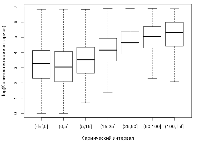
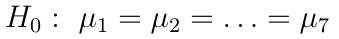
It can already be observed that with the growth of karma, the median of the number of comments that the user leaves also grows. Considering the above, our null hypothesis for analysis of variance can be formulated as follows: karma has no effect on the logarithm of the number of comments left by the user, and the observed differences between the group averages are insignificant and random:
An alternative hypothesis, respectively, argues that the differences are not accidental. To accept or reject the null hypothesis, we need to compare the intergroup VAR b and the intragroup VAR w dispersion. Both of these quantities estimate the dispersion of the general population in their own way, and with a valid null hypothesis, their ratio is close to 1, i.e intragroup and intergroup dispersions do not differ. The formulas for calculating these variances are given below:
Here K is the number of groups, N is the total sample size. Now we need to evaluate the ratio
In this context, it is customary to say that the value of F follows an F-distribution with degrees of freedom K-1 and NK. A small piece of code on R that computes the statistics F test and the critical value F crit at a level of significance α = 5%:
alpha <- 0.05 K <- length(levels(karma_cut)) N <- nrow(user_data) df1 <- K - 1 df2 <- N - K M <- mean(comments_log) var_b <- sum(tapply(comments_log, karma_cut, function(x){ length(x) * (mean(x) - M) ^ 2})) / df1 var_w <- sum(tapply(comments_log,karma_cut, function(x){ sum((x - mean(x))^2)})) / df2 Ftest <- var_b / var_w Fcrit <- qf(alpha, df1, df2, lower.tail=F) The graph below shows the distribution F (6, 14668), the critical and calculated statistics values:

Obviously, F crit << F test , which means that the hypothesis H 0 can be rejected. In R, of course, all of the above has long been implemented, so just check the calculation:
m.aov <- aov(comments_log ~ karma_cut) summary(m.aov) Df Sum Sq Mean Sq F value Pr(>F) karma_cut 6 5519 919.9 556.2 <2e-16 *** Residuals 14668 24260 1.7 --- Signif. codes: 0 '***' 0.001 '**' 0.01 '*' 0.05 '.' 0.1 ' ' 1 The value of F-statistics is 556.2, which coincides with the previously calculated.
Post hoc
Calculations show that the hypothesis H 0 about equality of averages should be rejected (this is the only thing we can say by running ANOVA). What to do with this conclusion next? Usually, post-hoc analysis is performed after ANOVA: you can use the t-test with the Bonferroni correction (in R it's pairwise.t.test ) or, for example, Tukey's HSD test to find out between which groups there are differences. I like the last test more:
TukeyHSD(m.aov, "karma_cut", conf.level=0.95) Tukey multiple comparisons of means 95% family-wise confidence level Fit: aov(formula = comments_log ~ karma_cut) $karma_cut diff lwr upr p adj (0,5]-(-Inf,0] -0.08189943 -0.17990408 0.01610521 0.1725558 (5,15]-(-Inf,0] 0.29578008 0.20925195 0.38230821 0.0000000 (15,25]-(-Inf,0] 0.92766799 0.81485590 1.04048009 0.0000000 (25,50]-(-Inf,0] 1.36762030 1.25442791 1.48081269 0.0000000 (50,100]-(-Inf,0] 1.66955943 1.53041195 1.80870691 0.0000000 (100, Inf]-(-Inf,0] 1.87283311 1.69233134 2.05333488 0.0000000 (5,15]-(0,5] 0.37767952 0.26881660 0.48654243 0.0000000 (15,25]-(0,5] 1.00956743 0.87883646 1.14029840 0.0000000 (25,50]-(0,5] 1.44951973 1.31846045 1.58057902 0.0000000 (50,100]-(0,5] 1.75145887 1.59742628 1.90549145 0.0000000 (100, Inf]-(0,5] 1.95473255 1.76252197 2.14694313 0.0000000 (15,25]-(5,15] 0.63188791 0.50952455 0.75425128 0.0000000 (25,50]-(5,15] 1.07184022 0.94912615 1.19455428 0.0000000 (50,100]-(5,15] 1.37377935 1.22678192 1.52077678 0.0000000 (100, Inf]-(5,15] 1.57705303 1.39043280 1.76367327 0.0000000 (25,50]-(15,25] 0.43995231 0.29748058 0.58242403 0.0000000 (50,100]-(15,25] 0.74189144 0.57803877 0.90574410 0.0000000 (100, Inf]-(15,25] 0.94516512 0.74499878 1.14533146 0.0000000 (50,100]-(25,50] 0.30193913 0.13782440 0.46605386 0.0000012 (100, Inf]-(25,50] 0.50521281 0.30483189 0.70559373 0.0000000 (100, Inf]-(50,100] 0.20327368 -0.01283281 0.41938017 0.0811265 It can be preliminarily concluded that users with karma (-∞, 0] and (0, 5] leave approximately the same log number of comments, as do users with karma (50,100] and (100, ∞]. The other groups differ significantly).
What's wrong?
We could stop at this, but there are a few comments in addition to what is under the spoiler above. First of all, you should pay attention to our "normalized" variable comments_log:
On closer examination, it turns out to be very far from the normal distribution, as the Shapiro-Wilk test hints at. Another criterion - the Bartlett test - indicates that the variance in groups is heterogeneous:
bartlett.test(comments_log~karma_cut) Bartlett test of homogeneity of variances data: comments_log by karma_cut Bartlett's K-squared = 84.811, df = 6, p-value = 3.613e-16 On the one hand, there is a violation of the prerequisites of ANOVA, on the other hand, there are a number of papers that say that analysis of variance is very resistant to the violation of the normality condition and the dispersion heterogeneity. If the violation of conditions is still constrained by someone, then you can use the non-parametric Kruskal-Wallis test. Here, the null hypothesis is the assumption of equality of the medians (and not the mean!) In all groups:
kruskal.test(comments_log ~ karma_cut) Kruskal-Wallis rank sum test data: comments_log by karma_cut Kruskal-Wallis chi-squared = 2816.1, df = 6, p-value < 2.2e-16 The Kruskal-Wallis test also allows you to reject the null hypothesis. Since the Kruskal-Wallis test is non-parametric, then the post-hoc analysis must also be based on non-parametric tests, such as, for example, the Mann-Whitney U-test with the subsequent correction of p-values, the Dunn test. The latter is contained in the R dunn.test package:
dunn.test::dunn.test(comments_log, karma_cut, method="bonferroni") 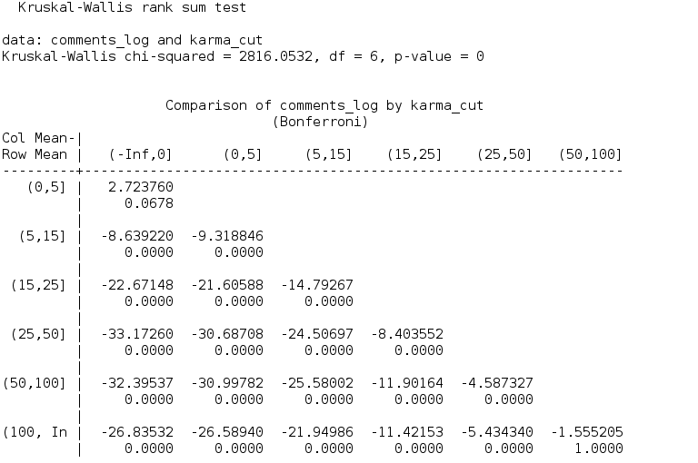
At the 5% level of significance, like the Tukey test, Dunn's criterion says that users with karma (-∞, 0] and (0, 5], and (50,100] and (100, ∞]. Leave approximately the same log- number of comments.
ANOVA and linear regression
Speaking of analysis of variance, it is impossible not to mention the linear regression. Moreover, it can be argued that this is practically the same thing, since The analysis of variance model is a special case of linear regression. We write the linear regression with the factor variable and check its coefficients:
m.lm <- lm(comments_log ~ karma_cut-1) summary(m.lm) Coefficients: Estimate Std. Error t value Pr(>|t|) karma_cut(-Inf,0] 3.20288 0.01736 184.50 <2e-16 *** karma_cut(0,5] 3.12098 0.02834 110.12 <2e-16 *** karma_cut(5,15] 3.49866 0.02366 147.88 <2e-16 *** karma_cut(15,25] 4.13055 0.03409 121.16 <2e-16 *** karma_cut(25,50] 4.57050 0.03424 133.50 <2e-16 *** karma_cut(50,100] 4.87244 0.04388 111.04 <2e-16 *** karma_cut(100, Inf] 5.07571 0.05870 86.47 <2e-16 *** --- Signif. codes: 0 '***' 0.001 '**' 0.01 '*' 0.05 '.' 0.1 ' ' 1 Residual standard error: 1.286 on 14668 degrees of freedom Multiple R-squared: 0.8914, Adjusted R-squared: 0.8913 F-statistic: 1.719e+04 on 7 and 14668 DF, p-value: < 2.2e-16 Now we find the average number of log comments for each karmic slice:
tapply(comments_log, karma_cut, mean) (-Inf,0] (0,5] (5,15] (15,25] (25,50] (50,100] (100, Inf] 3.202879 3.120979 3.498659 4.130547 4.570499 4.872438 5.075712 The coefficients in linear regression are the mean values, i.e. the following formula is valid:

where μ i is the average of the corresponding group, ε ij is a random error distributed normally.
Conclusion
So, the variance analysis is performed according to the following scheme:
- The dependent and factor variables are determined.
- Prerequisites for ANOVA are checked.
- With a normal dependent variable and homogeneous dispersion, ANOVA is performed; otherwise, the non-parametric Kruskal-Wallis test
- After analyzing the variance and rejecting the null hypothesis, the appropriate post-hoc analysis is performed - parametric or non-parametric.
In the multivariate analysis of dispersions , the F-test is also used, but the formulas for calculating the variance are complicated; in addition, there are additional terms that describe the interaction between factors, and several null hypotheses appear.
As for the comments on Habré, both ANOVA and the Kruskal-Wallis test say that there is a relationship between the log number of comments and the user's karma, with groups with karma (-∞, 0] and (0, 5], and (50,100] and (100, ∞] leave approximately the same number of comments. In general, as the karma itself grows, the number of comments increases. Interestingly, the results of both non-parametric and parametric tests coincided, although the prerequisites for the latter were clearly violated. This fact can be explained robustness analysis of variance a, and the fact that with a large amount of data (we have thousands of measurements), the violation of the assumption that the data is normal has a much smaller effect on the result than in the case of a small sample.
Source: https://habr.com/ru/post/304528/
All Articles