Search for connections in social networks
Hi, Habr! In this post we want to share our solution to the problem of predicting hidden connections in the Beeline corporate social network “Beehive”. We solved this task in the framework of the Microsoft virtual hackathon. I must say that before this hackathon, our team already had successful experience in solving such tasks on the hackathon from Odnoklassniki and we really wanted to try out our developments on new data. In the article we will tell about the main approaches that are used in solving such problems and share the details of our solution.
Development of a high-quality algorithm for recommending friends is one of the top priorities for almost any social network because This functionality is a powerful tool to engage and retain users.
In the English literature there are quite a lot of publications on this topic, and the task itself even has a special abbreviation PYMK (People You May Know).
The Beeline company in the framework of the virtual hackathon from Microsoft provided the graph of the corporate social network "Beehive". 5% of the edges in the graph was artificially hidden. The task was to find the hidden edges of the original graph.
')
In addition to having a connection between social network users, for each pair, information was also provided on the companies in which the users work, information on the number of sent and received messages, the duration of calls and the number of sent and received documents.
The problem of searching for edges is formulated as a binary classification problem, and the measure F1 was proposed as an acceptance metric. In some such tasks, the quality metric is considered separately for each user and the average is evaluated. In this task, the quality was evaluated globally for all edges.
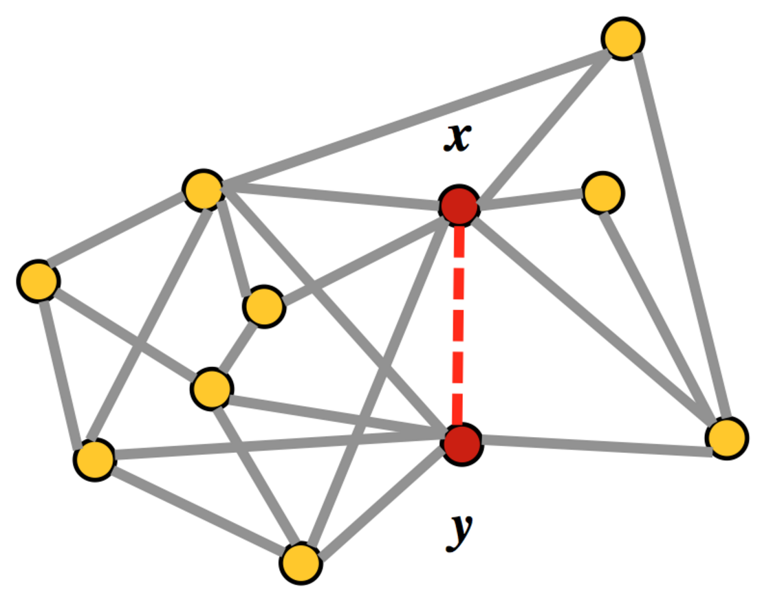
In the general case, to search for hidden edges in a graph, it is necessary to iterate all possible pairs of vertices and for each pair to obtain an estimate of the probability of a link.
For large graphs, this approach will require a lot of computational resources. Therefore, in practice, many candidates in social graphs are limited only to pairs that have at least one friend in common. As a rule, such a restriction allows to significantly reduce the amount of computation and speed up the work of the algorithm without a significant loss in quality.
Each pair of candidates is described by a feature vector and a binary answer: “1” if there is an edge or “0” if there is no edge. On the obtained set {feature vector, answer}, a model is taught that predicts the probability of the presence of an edge for a pair of candidates.
Since if the graph in this problem is not directed, then the feature vector should not depend on the rearrangement of candidates in the pair. This property allows for training to take into account a couple of candidates only once and to reduce the size of the training sample by half.
To answer the question of exactly which edges are hidden in the original graph, the probability estimate at the output of the model must be turned into a binary answer, choosing the appropriate threshold value.
To assess the quality and selection of model parameters, we removed 5% of randomly selected edges from the provided graph. The remaining graph was used to search for candidates, generate traits and train the model. Hidden edges used for the selection of the threshold and the final quality assessment.
The following describes the main approaches for generating features in the PYMK task.
For each user, we consider statistics: the distribution of friends by geography, community, age or sex. Using these statisticians, we obtain an estimate of the similarity of the candidates to each other, for example, using a scalar product.
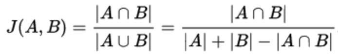
Jacquard Coefficient - allows you to evaluate the similarity of the two sets. As sets there can be friends as well, for example, and communities of candidates.
The Adamik / Adar coefficient is essentially a weighted sum of the mutual friends of the two candidates.
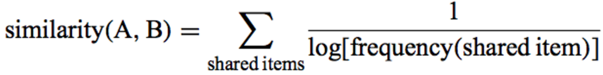
The weight in this amount depends on the number of friends of the mutual friend. The less friends a mutual friend has, the greater his contribution to the resulting amount. By the way, we actively used this idea in our decision.
These features are the result of matrix expansions. Moreover, expansions can be applied both to the matrix of relations between users, and to the community matrix — the user, or geography — the user and the like. The resulting decomposition of a vector with latent signs can be used to assess the similarity of objects to each other, for example, using a cosine distance measure .
Perhaps the most common algorithm for matrix decomposition is SVD . You can also use ALS and the community search algorithm in BigCLAM graphs, which is popular in recommender systems.
This group of signs is calculated taking into account the structure of the graph. As a rule, to save time, not the entire graph is used in calculations, but some of it, for example, a subgraph of common friends of depth 2.
One of the popular signs is Hitting Time - the average number of steps required to pass a route from one candidate to another, taking into account the weights of the ribs. The path is laid in such a way that the next vertex is chosen randomly with a probability depending on the values of the attributes of the edges emanating from the current node.
In solving this problem, we actively used the idea of the Adamyk / Adar coefficient that not all friends are equally useful. We experimented with the discounting function - we tried fractional degrees instead of the logarithm, and we also experimented with weighing common friends on various utility attributes.
Since we worked on the task in parallel, then we got two independent solutions, which were later combined for the final submission.
The first solution is based on the Adamik / Adar idea and is an empirical formula that takes into account both the number of friends of a common friend and the flow of messages between candidates through mutual friends.
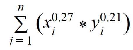
n is the number of mutual friends;
xi - the number of friends in a common friend;
yi is the sum of incoming and outgoing messages between candidates through their mutual friend
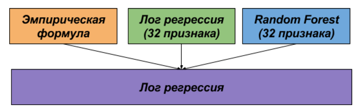
In the second solution, we generated 32 signs and trained on them the log model. regression and random forest.
The models from the first and second solutions were combined using another logistic regression.
The table describes the main features that were used in the second solution.
The table below shows the quality ratings of both the individual and the resulting models.
So, the model is trained. The next step is to select a threshold to optimize the acceptance metric.
In this problem, we optimized the F1 metric.
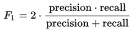
This metric is equally sensitive to both accuracy and completeness and is the harmonic average of these values.
Since the dependence of the F1 metric on the threshold is a convex function, then the search for the maximum is not difficult.
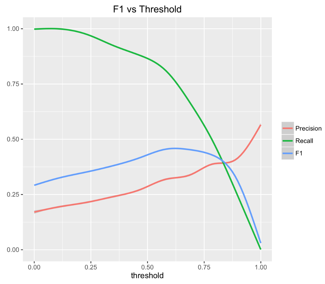
In this problem, we used the binary search algorithm to select the optimal threshold value.
The source graph was defined as a list of edges with the identification of users and the corresponding attributes. A total of 5.5 million links were represented in the training sample. The source data is provided in the form of a text file in the csv format and occupy 163Mb on the hard disk.
As part of the hackathon, we were provided with Azure cloud service resources under the Microsoft BizSpark program, in which we created a virtual machine for our calculations. The server price per hour was $ 0.2 and did not depend on the intensity of the calculations. The budget allocated by the organizers was enough to solve this problem.

We implemented the search algorithm for common friends on Spark, the results of intermediate calculations were cached to disk in parquet format, which significantly reduced the time for reading data. The running time of the search algorithm for common friends in a virtual machine was 8 hours. Candidates with a list of common friends in the parquet format occupy 2.1GB.
The algorithm for learning and selecting model parameters is implemented in python using the scikit-learn package. The processes of generating features, learning the model and selecting the threshold on a virtual server took about 3 hours in total.
In conclusion, I would like to thank Ivan Bragin for his active participation in solving the problem and his creativity in choosing the empirical formula.
Task setting and baseline data
Development of a high-quality algorithm for recommending friends is one of the top priorities for almost any social network because This functionality is a powerful tool to engage and retain users.
In the English literature there are quite a lot of publications on this topic, and the task itself even has a special abbreviation PYMK (People You May Know).
The Beeline company in the framework of the virtual hackathon from Microsoft provided the graph of the corporate social network "Beehive". 5% of the edges in the graph was artificially hidden. The task was to find the hidden edges of the original graph.
')
In addition to having a connection between social network users, for each pair, information was also provided on the companies in which the users work, information on the number of sent and received messages, the duration of calls and the number of sent and received documents.
The problem of searching for edges is formulated as a binary classification problem, and the measure F1 was proposed as an acceptance metric. In some such tasks, the quality metric is considered separately for each user and the average is evaluated. In this task, the quality was evaluated globally for all edges.
Training and test
In the general case, to search for hidden edges in a graph, it is necessary to iterate all possible pairs of vertices and for each pair to obtain an estimate of the probability of a link.
For large graphs, this approach will require a lot of computational resources. Therefore, in practice, many candidates in social graphs are limited only to pairs that have at least one friend in common. As a rule, such a restriction allows to significantly reduce the amount of computation and speed up the work of the algorithm without a significant loss in quality.
Each pair of candidates is described by a feature vector and a binary answer: “1” if there is an edge or “0” if there is no edge. On the obtained set {feature vector, answer}, a model is taught that predicts the probability of the presence of an edge for a pair of candidates.
Since if the graph in this problem is not directed, then the feature vector should not depend on the rearrangement of candidates in the pair. This property allows for training to take into account a couple of candidates only once and to reduce the size of the training sample by half.
To answer the question of exactly which edges are hidden in the original graph, the probability estimate at the output of the model must be turned into a binary answer, choosing the appropriate threshold value.
To assess the quality and selection of model parameters, we removed 5% of randomly selected edges from the provided graph. The remaining graph was used to search for candidates, generate traits and train the model. Hidden edges used for the selection of the threshold and the final quality assessment.
The following describes the main approaches for generating features in the PYMK task.
Counters
For each user, we consider statistics: the distribution of friends by geography, community, age or sex. Using these statisticians, we obtain an estimate of the similarity of the candidates to each other, for example, using a scalar product.
Similarity sets and common friends
Jacquard Coefficient - allows you to evaluate the similarity of the two sets. As sets there can be friends as well, for example, and communities of candidates.
The Adamik / Adar coefficient is essentially a weighted sum of the mutual friends of the two candidates.
The weight in this amount depends on the number of friends of the mutual friend. The less friends a mutual friend has, the greater his contribution to the resulting amount. By the way, we actively used this idea in our decision.
Latent factors
These features are the result of matrix expansions. Moreover, expansions can be applied both to the matrix of relations between users, and to the community matrix — the user, or geography — the user and the like. The resulting decomposition of a vector with latent signs can be used to assess the similarity of objects to each other, for example, using a cosine distance measure .
Perhaps the most common algorithm for matrix decomposition is SVD . You can also use ALS and the community search algorithm in BigCLAM graphs, which is popular in recommender systems.
Signs on graphs
This group of signs is calculated taking into account the structure of the graph. As a rule, to save time, not the entire graph is used in calculations, but some of it, for example, a subgraph of common friends of depth 2.
One of the popular signs is Hitting Time - the average number of steps required to pass a route from one candidate to another, taking into account the weights of the ribs. The path is laid in such a way that the next vertex is chosen randomly with a probability depending on the values of the attributes of the edges emanating from the current node.
Decision
In solving this problem, we actively used the idea of the Adamyk / Adar coefficient that not all friends are equally useful. We experimented with the discounting function - we tried fractional degrees instead of the logarithm, and we also experimented with weighing common friends on various utility attributes.
Since we worked on the task in parallel, then we got two independent solutions, which were later combined for the final submission.
The first solution is based on the Adamik / Adar idea and is an empirical formula that takes into account both the number of friends of a common friend and the flow of messages between candidates through mutual friends.
n is the number of mutual friends;
xi - the number of friends in a common friend;
yi is the sum of incoming and outgoing messages between candidates through their mutual friend
In the second solution, we generated 32 signs and trained on them the log model. regression and random forest.
The models from the first and second solutions were combined using another logistic regression.
The table describes the main features that were used in the second solution.
| sign | description |
|---|---|
| Analogue of the Adamik / Adar coefficient, but instead of the logarithm a third degree root was used | |
| We weigh mutual friends with the conductivity of messages. The smaller the ratio of outgoing and incoming messages / calls / documents of a common friend, the higher its weight when summing up | |
| flow_common | We evaluate the permeability of messages / calls / documents between candidates through a mutual friend. The higher the permeability, the greater the weight in the summation |
| friends_jaccard | Jacquard coefficient for friends of candidates |
| friend_company | Similarity based on the share of friends of the user from the candidate’s company |
| company_jaccard | We evaluate the friendliness of candidate companies using the Jacquard coefficient (equal to one if the candidates are from the same company) |
The table below shows the quality ratings of both the individual and the resulting models.
| Model | F1 | Accuracy | Completeness |
|---|---|---|---|
| Empirical formula | 0.064 | 0.059 | 0.069 |
| Log regression | 0.060 | 0.057 | 0.065 |
| Random forest | 0.065 | 0.070 | 0.062 |
| Log regression + Random Forest | 0.066 | 0.070 | 0.063 |
| Log regression + Random Forest + Empirical formula | 0.067 | 0.063 | 0.071 |
Threshold selection
So, the model is trained. The next step is to select a threshold to optimize the acceptance metric.
In this problem, we optimized the F1 metric.
This metric is equally sensitive to both accuracy and completeness and is the harmonic average of these values.
Since the dependence of the F1 metric on the threshold is a convex function, then the search for the maximum is not difficult.
In this problem, we used the binary search algorithm to select the optimal threshold value.
Technology
The source graph was defined as a list of edges with the identification of users and the corresponding attributes. A total of 5.5 million links were represented in the training sample. The source data is provided in the form of a text file in the csv format and occupy 163Mb on the hard disk.
As part of the hackathon, we were provided with Azure cloud service resources under the Microsoft BizSpark program, in which we created a virtual machine for our calculations. The server price per hour was $ 0.2 and did not depend on the intensity of the calculations. The budget allocated by the organizers was enough to solve this problem.
We implemented the search algorithm for common friends on Spark, the results of intermediate calculations were cached to disk in parquet format, which significantly reduced the time for reading data. The running time of the search algorithm for common friends in a virtual machine was 8 hours. Candidates with a list of common friends in the parquet format occupy 2.1GB.
The algorithm for learning and selecting model parameters is implemented in python using the scikit-learn package. The processes of generating features, learning the model and selecting the threshold on a virtual server took about 3 hours in total.
In conclusion, I would like to thank Ivan Bragin for his active participation in solving the problem and his creativity in choosing the empirical formula.
Source: https://habr.com/ru/post/303838/
All Articles