Methodical notes on the selection of informative features (feature selection)
Hello!
My name is Alexei Burnakov. I am a Data Scientist at Align Technology. In this article I will tell you about the approaches to the feature selection, which we practice in the course of experiments on data analysis.
In our company, statistics and machine learning engineers analyze large volumes of clinical information related to the treatment of patients. In a nutshell, the meaning of this article can be reduced to extracting valuable bits of knowledge contained in a small fraction of noisy and redundant gigabytes of data available to us.
')
A source.
It has been established that sets with a large number of input variables may contain redundant information and lead to the re-learning of machine learning models if the regularizer is not built into the models. The stage of selection of informative features ( IPR here and below) is often a necessary step in preprocessing data during an experiment.
The experiments carried out in the article do not pretend to scientific completeness due to the fact that analytical justifications for the optimality of a particular method will not be given, and the reader is referred to the original sources for more detailed and mathematically accurate presentation. In addition, the disclaimer is that on other data the value of a particular method will change, which makes the task as a whole intellectually attractive.
At the end of the article, the results of the experiments will be summarized and a reference to the full R code on Git will be made.
I express my gratitude to all the people who read the material before publication and made it better, in particular, to Vlad Shcherbinin and Alexei Seleznev.
Let's look at the general approach to classifying IPR methods by referring to the wiki:
A source.
Examples
The wrapping algorithm of the IPR can be called a combination of methods, including searching for a subset of input variables followed by training, for example, random forest, on selected data and evaluating its error in cross-training. That is, for each iteration, we will train the whole machine (already actually ready for further use).
Filtering algorithm IPRs can be called enumeration of input variables, complemented by conducting a statistical test for the relationship between the selected variables and the output. If our inputs and output are categorical, then it is possible to conduct a chi-square test for independence between an input (or a combined set of inputs) and an output with a p-value estimate and, as a consequence, a binary conclusion about the significance or insignificance of the selected set of features. Other examples of filtering algorithms include:
The built-in IPR algorithm is, for example, p-values corresponding to linear regression coefficients. In this case, p-value also allows you to make a binary conclusion about a significant difference in the coefficient from zero. If you scale all the inputs of the model, the modules of the scales can be interpreted as indicators of importance. You can also use the R ^ 2 model - a measure of explaining the variance of a process with simulated values. Another example is the function of assessing the importance of input variables, built-in random forest. In addition, weights modules can be used that correspond to the inputs in an artificial neural network. This list is not exhausted.
At this stage, it is important to understand that this distinction, in fact, indicates a difference in the fitness functions of the IPR, that is, a measure of the relevance of the found subset of input features in relation to the problem being solved. Subsequently, we will return to the question of choosing a fitness function.
Now, when we are a little oriented in the main groups of methods of IPRs, I suggest paying attention to what methods are used to iterate over the subsets of input variables. Turn again to the wiki page:
A source.
I deliberately did not translate the names of some algorithms, since I was not familiar with their Russian-language interpretation.
The search for a subset of predictors is a discrete problem, since at the output we get a vector of integers, denoting input indices, of the form:
inputs: 1 2 3 4 5 6 ... 1000
Selection: 0 0 1 1 1 0 ... 1
We will return to this feature later and illustrate where it leads in practice.
The result of the whole experiment strongly depends on how the search for a subset of input features is configured. In order to intuitively understand the main difference in these approaches, I suggest the reader to divide them into two groups: greedy (non-greedy) and non-greedy.
They are used often, as they are fast and give a good result in many tasks. The greed of the algorithm is that if one of the candidates for entry into the final subset was chosen (or excluded), then it remains in it (in the case of a greedy inclusion) or forever absent (in the case of a greedy exception). Thus, if candidate A was selected at early iterations, at later iterations a subset will always include him and other candidates, which, together with A, show an improvement in the metric of importance of the subset for the output variable. The opposite situation is for exclusion: if candidate A was removed, because after his exclusion, the importance metric is least affected or improved, the researcher will not receive information about the importance metric, where A is in the subset and other candidates excluded later.
If we draw a parallel with the search for a maximum (minimum) in multidimensional space, the greedy algorithm will get stuck in a local minimum, if there is one, or quickly find the optimal solution, if there is a single minimum, and it is global.
On the other hand, enumeration of all greedy variants is carried out relatively quickly and allows to take into account some interactions between inputs.
Examples of greedy algorithms: greedy inclusion (forward selection; step forward) and greedy exception (backward elimination; step backward). The list is not limited to this.
The principle of operation of non-greedy algorithms implies the ability to discard all or partly formed subsets of features, combinations of subsets among themselves and make random changes to the subsets in order to avoid a local minimum.
If we draw an analogy with the search for the maximum (minimum) values of the fitness function in a multidimensional space, non-greedy algorithms consider much more neighboring points and can even make large jumps to random areas.
It is possible to present graphically the operation of these types of algorithms.
First, the greedy inclusion:

Now non-greedy - stochastic - search:
In both cases, you need to select one of the best combination of two inputs, whose indices are plotted along the axes of the graph. The greedy algorithm begins by selecting the one best entry, going through the indexes horizontally. And then adds a second input to the selected input so that their total relevance is maximum. But it turns out that of all possible combinations, it completely passes only 1/37 part. When you add another dimension, the number of cells traversed will become even smaller: approximately 1/3 ^ 2.
In this case, a practical situation is possible when the wrong combination is not the one that the greedy algorithm found. This can occur if each of the two inputs separately does not show the best relevance to the task (and they will not be selected in the first step), but their interaction maximizes the relevance metric.
The rash algorithm seeks much longer:
and checks for more possible combinations of inputs. But he has a chance to find, perhaps, an even better subset of inputs due to a sweeping search at once in all changes of the task.
There are search algorithms that go beyond the established greedy / non-greedy dichotomy.
An example of such a separate search would be to iterate through the inputs individually and evaluate their individual importance for the output variable. With this, by the way, the first wave begins in the greedy variable inclusion algorithm. But what is good with such a search, except that it is very fast? Each input variable begins to exist "in a vacuum", that is, without taking into account the influence of other inputs on the connection between the selected input and output. At the same time, after the completion of the algorithm, the resulting list of inputs indicating their individual importance for the output only gives information about the individual significance of each predictor. When combining a number of the most important predictors, according to this list, you can get a number of problems:
As you can see, the problems are not the most trivial.
The main question in the problem of the IPR is formulated as the optimal combination of the subset search method and the fitness function.
Let us consider this statement in more detail. Our problem of IPR can be described by two hypotheses:
a) the surface of the error is simple or complex;
b) there are simple or complex dependencies in the data.
Depending on the answers to these questions, the choice should be made on a specific combination of the search method and the method for determining the relevance of the selected characteristics.
Surface error.
An example of a simple surface:
A source.
Here we choose a combination of two inputs, determining their relevance to the output and descend along a smooth surface in the direction of the gradient, almost certainly at the optimum point.
An example of a complex surface:

A source.
In this case, solving the same problem, we encounter a set of local minima, the greedy algorithm cannot get out of which. At the same time, the algorithm with a stochastic search has an increased chance of finding a more accurate solution.
We mentioned earlier that finding a subset of predictors is a discrete task. If the dependence of the output on the inputs includes interactions, when moving from one point of space to the next one, one can observe sharp jumps in the value of the fitness function. The surface error in our case is often not smooth, not differentiable:
This is an example of finding a subset of two inputs and the corresponding value of the relevance function of a subset of the output variable. It can be seen that the surface is far from smooth, with peaks, and also includes a rugged plateau of approximately the same values. Nightmare for methods of greedy gradient descent.
Dependencies
As the number of measurements of a task grows, the theoretical chance increases that the dependence of the output variable has a very complex structure and involves many inputs. In addition, the dependence can be either linear or non-linear. If the dependence implies the interaction of predictors and a non-linear form, it will be possible to find it only taking into account both these points, applying, for example, random forest or neural network training. If the dependence is simple, linear, includes only a small part of all the predictors, the approach to finding it - and, as a result, to the IPR - can be reduced to alternate inclusion in the linear regression model with 1 or more inputs with a model quality rating.
An example of a simple dependency:
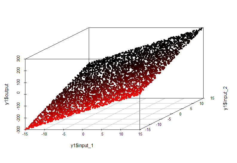
In this case, the dependence of the value along the output axis on the values input1 and input2 is described by a plane in space:
The model of such dependence is very simple and can be approximated by linear regression.
An example of a complex dependency:
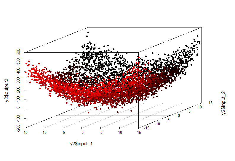
This non-linear relationship can no longer be detected by the construction of a linear model. Her appearance is:
It is also necessary to take into account the dimension of the problem.
If the number of input variables is large, the search for the optimal subset by stochastic (non-greasy) methods can be very expensive due to the fact that the total number of all possible subsets is given by
Accordingly, the search for a minimum in such a variety can be very long. On the other hand, the use of a greedy search will make it possible to make a first approximation in a reasonable time, even if it is a local minimum and the researcher will know about it.
In the absence of objective knowledge about the phenomenon under study, it is impossible to say in advance how complex the dependence of input variables and output will be and how many inputs will be optimal for finding an approximate or exact solution to the problem of selecting the optimal subset of inputs. It is also difficult to predict whether the surface of the error during the IPR is smooth and simple or complex and rugged.
We are also always limited in resources and must make the most optimal decisions. As a small help in developing an approach to IPR, you can use the following table:

Thus, we always have the opportunity to consider several combinations of methods for finding a subset of inputs and the fitness function of relevance. The most expensive and probably the most effective combination is the greedy search and wrapper fitness wrapping. It allows you to avoid a local minimum, while providing the most accurate measure of the relevance of the selected inputs, since at each iteration there is a trained model (and its accuracy for validation).
The least expensive, but not always the least effective approach, is a greedy search paired with a filter function, which can be a statistical test, a correlation coefficient, or a quantity of mutual information.
In addition, the embedded (embedded) methods allow immediately after training the model to weed out a number of inputs that are unnecessary from the algorithm algorithm point of view, without losing significantly the accuracy of the simulation.
A good way is to try to solve a problem several times in different ways and choose the best one.
In general, the selection of informative features is the selection of the best combination of the multi-dimensional search method and the most optimal fitness function of the relevance of the selected subset with respect to the output variable.

A source.
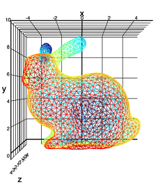
Our experimental data set ("Stanford rabbit"):

I just love rabbits.
We will look at the dependence of the height of a point (Z axis) on latitude and longitude. In this case, I add 10 noise variables to the set with a distribution approximately corresponding to the mixture of two informative inputs (X and Y), but not related to the variable Z.
Let's look at histograms of the density of distribution for the variables X, Y, Z and one of the noise variables.
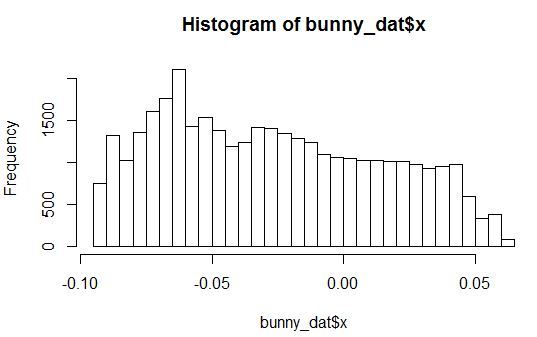
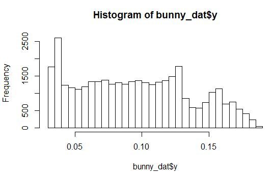

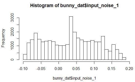
It is seen that the distribution with arbitrary parameters. In this case, all noise variables are distributed in such a way that they have a small peak in a certain range of values.
Further, the data set will be randomly divided into two parts: training and validation.
Data preparation.
Experiment №1: greedy search for a subset of inputs with a linear function of assessing importance (as the fitness function, the variant wrapper will be used - an estimate of the coefficient of determination of a trained model on a validation sample).
Result:
It turned out to include noise variables.
Let's look at the trained model:
We see that in fact, only our original inputs and the free term of the equation take statistical significance.
And now let's get the greedy exception of variables.
Result:
The model also included noises.
Let's look at the trained model:
Similarly, inside the model, we see that only the original inputs are important.
If we train the model only on variables X and Y, we get:
The fact is that the validation of R ^ 2 was higher when the noise variables were turned off.
Strange result! Probably, because of the data structure, the noise does not have a detrimental effect on the model.
But we have not tried to take into account the interaction of predictors.
It turned out well:
The interaction of X and Y is significant. What about R ^ 2 on validation?
This is the highest value we have seen. Unfortunately, it was the interaction option that was not incorporated into the fitness function and we missed this combination of inputs.
Experiment number 2: the greedy search for a subset of inputs with a linear function of assessing the importance (as the fitness function will be used the option embedded - f-statistics of the trained model on the training set).
The result of the sequential inclusion of variables is only one predictor Y. For it, F-Statistic was maximized. That is, this variable is very important. But for some reason, the variable X is forgotten.
And now the sequential elimination of variables.
The result is similar - only one variable Y.
It can be noted that while maximizing the F-Statistic multi-variable model, all the noise turned out to be overboard, and the model turned out to be robust: the coefficient of determination for validation is almost as good as the best model from experiment No. 1:
Experiment No. 3: sequential assessment of the individual significance of predictors using the Pearson correlation coefficient (this option is the simplest, it does not take into account the interaction, the fitness function is also simple — it evaluates only the linear relationship).
Result:
The largest correlation is Z with Y, and in second place is X. However, correlation X is not explicitly expressed and requires a statistical test for the significance of the difference in the correlation coefficient from zero for each of the variables.
On the other hand, in all 3 experiments we did not take into account the interaction of predictors (X * Y) at all. This may explain the fact that the estimation of single significance or the linear inclusion of predictors in the equation does not give us an unequivocal answer.
Such an experiment:
Indicates that the interaction of X and Y correlates with Z quite strongly.
Experiment number 4: assessment of the importance of predictors by the algorithm embedded in the machine (the variant of the greedy search and the embedded fitness function of the importance of inputs into GBM).
We will train Gradient Boosted Trees (gbm) and look at the importance of variables. Good article detailing aspects of using GBM: Gradient boosting machines, a tutorial.
Take the learning parameters from the ceiling, set a very low learning rate to avoid strong retraining. Note that any decision trees are greedy, and improving the model by adding many models is achieved by sampling observations and inputs.
Result:
This approach perfectly coped with the task and singled out noiseless inputs, making all other inputs absolutely insignificant.
Moreover, it should be noted that the setup of this experiment is very fast, everything works almost out of the box. More careful planning of this experiment, including cross-training to obtain optimal learning parameters, is more difficult, but this is necessary when preparing a real model in production.
Experiment # 5: assessing the importance of predictors using a stochastic search with a linear importance rating function (this is a non-greasy search in the input space, and the wrapper variant will be used as the fitness function — an estimate of the determination coefficient of the trained model on the validation sample).
This time, the learning linear model involves pairwise interactions between the predictors.
What happened?
We see that we miss. Noise included.
As you can see, the best value of the coefficient of determination for validation is achieved with the inclusion of noise variables. In this case, the convergence of the search algorithm is exhaustive:

Let's try to change the fitness function, save the search method.
Experiment # 6: assessing the importance of predictors using a stochastic search with a linear function of assessing importance (this is a non-greasy search in the space of inputs, the fitness function is the embedded p-values corresponding to the coefficients of the model).
We will select a set of predictors that minimize the average p-value of the coefficients in the model.
Result:
This time everything worked out. Only original predictors were selected, since their p-values are really small.
The algorithm convergence is good in 60 seconds:
Experiment number 7: assessing the importance of predictors using a greedy search with an assessment of the importance of the quality of the trained model (this is a greedy search in the input space, the fitness function is a wrapper corresponding to the determination coefficient on the validation of the boosted decision trees model).
Result with greedy predictors:
Got the point!
Result with the greedy exception of predictors:
It's getting worse. The inclusion of noise predictors in the model did not greatly impair the quality of the prediction on validation. And there is an explanation for this: random decision forests have a built-in regularizer and can themselves ignore non-informative inputs in the learning process.
This concludes the section of experiments on IPRs on standard methods. And in the next section, I will substantiate and show practical application, in my opinion, statistically reliable and doing a good job, based on information metrics.

A source.
We need to start with the concept of informational entropy. Entropy (Shannon) is a synonym for uncertainty. The more uncertain we are about the value of a random variable, the more entropy (another synonym for information) is the realization of this value. If we consider the example of tossing a coin, then the symmetric coin of all any other variants of coins will have the greatest entropy, because we have the greatest uncertainty in the next outcome of a toss.
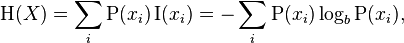
Formula for Shannon's entropy:
Suppose we flip a coin a few times. Can we say that our uncertainty about the next outcome of the throw diminished after we saw the result of the previous throw?
Suppose we have a coin that lands with an eagle with a probability of 2/3 after falling heads, and vice versa - after falling of an eagle, it lands on heads with a probability of 2/3. At the same time, the unconditional frequency of the fallouts of the eagle and tails remains 50/50.
For such a coin after a falling eagle, the frequency of tails is no longer 1/2, and vice versa. So, our uncertainty about the next outcome of the throw has decreased (we don’t expect 50/50).
To understand the phenomenon of dependence, we recall that probability theory defines independence as follows:
thus, the probability of the joint realization of events is equal to the product of the probabilities of their own realizations.
If this is observed, the events are independent in a mathematical sense. If
then events are not mathematically independent.
The same principle underlies the formula for measuring the relationship between two (and more) random variables in information theory.
We emphasize that here dependence is understood in a probabilistic sense. The analysis of causality requires a more comprehensive review, including both the analysis of false correlations and redundancy (through the use of mutual information), and the involvement of expert knowledge about the object under study.
You can also output mutual information through entropies:
In simple words, mutual information is the amount of entropy (uncertainty) that leaves the system, if there is a predictive variable (or several variables). For example, the entropy of a random variable is 3 bits. Mutual information is 2 bits. Hence, by 2/3, the uncertainty about the implementation of a random variable is compensated by the presence of a predictor.
Mutual information has the following properties:
Mutual information satisfies some of the requirements for the ideal measure of dependence, formulated in:
There is one property of mutual information ( VI ) that is useful to know when applying this measure:
This means that if our input variable has an entropy of 10 bits, and the output variable has 3 bits, then the maximum information that the input variable can transmit to the output is 3 bits. This is the maximum VI, which can be in such a system.
Another option is that the input variable has an entropy of 3 bits, and the output is 10 bits. The maximum information that an input can carry to the output is 3 bits, and this is the possible maximum of the VI.
If the VI value is divided by the entropy of the dependent variable, we get a value in the range [0, 1], which, by analogy with the correlation coefficient, indicates how, without taking into account the scale of values, the input variable determines the dependent variable.
There are a number of arguments for using VIs, although it involves a number of tradeoffs:
, , . , , , .
— (Multiinformation) (Total Correlation).
A source:
:

:
( ) , . , ( 1 n) ( 1 m), . , - .
, .
, , . :
.
, , :
, , , , .
, n N.
. , .
100 .
1000 .
, , .
, , . , . .:
1.
2.
, , . . , ( ). , .
, .
. . , , . .
( ), .
. . , , , . , 1 000 51% , - . . .
«» . — , :
, , , , , n , n 100. , , , .
, , .
, , ( ), :
, . .
, : , .
17 973 , 12 , 5 . , 3,226.
, 0,731.
?
3 . , 5 ^ 3,226 178 , 100 .
.
№8 , () ( , - — ).
0,9 ( ) 10 -, 1 1 ( ). 10 .
Result:
. . — .
20 , - 1 .
Result:
— .
18% . .
( ):
Minimum-redundancy-maximum-relevance (mRMR)
. :
«Feature selection based on mutual information: criteria of max-dependency, max-relevance, and min-redundancy,»
Hanchuan Peng, Fuhui Long, and Chris Ding
IEEE Transactions on Pattern Analysis and Machine Intelligence,
Vol. 27, No. 8, pp.1226-1238, 2005
, ( ) . .
() , () .
() , , , . , .
() , . , ( ).
, , , , , ( ) , . , mRMR , .
() , — limited sampling bias.
mRMR . , , , , .
.

, , GBM, p-values .
, . , , , . , XY-Noise1 . , ( ), Align Technology. , , , Gradient Boosted Trees ( . ).
, , , . , , , , .
, , . . , , .
. , , , , . , .
github: Git
My name is Alexei Burnakov. I am a Data Scientist at Align Technology. In this article I will tell you about the approaches to the feature selection, which we practice in the course of experiments on data analysis.
In our company, statistics and machine learning engineers analyze large volumes of clinical information related to the treatment of patients. In a nutshell, the meaning of this article can be reduced to extracting valuable bits of knowledge contained in a small fraction of noisy and redundant gigabytes of data available to us.
')
This article is intended for statisticians, machine learning engineers and specialists who are interested in finding dependencies in datasets. Also, the material presented in the article may be of interest to a wide circle of readers who are not indifferent to data mining. The material will not address the issues of feature engineering and, in particular, the application of such methods as the analysis of the main components.
A source.
It has been established that sets with a large number of input variables may contain redundant information and lead to the re-learning of machine learning models if the regularizer is not built into the models. The stage of selection of informative features ( IPR here and below) is often a necessary step in preprocessing data during an experiment.
- In the first part of this article, we will review some of the methods for selecting attributes and consider the theoretical points in this process. This section is rather a systematization of our views.
- In the second part of the article, we will experiment with an example of an artificial data set with the selection of informative features and make a comparison of the results.
- In the third part, we will highlight the theory and practice of using measures from information theory as applied to the problem under discussion. The method presented in this section is new, but it still requires numerous checks on various data sets.
The experiments carried out in the article do not pretend to scientific completeness due to the fact that analytical justifications for the optimality of a particular method will not be given, and the reader is referred to the original sources for more detailed and mathematically accurate presentation. In addition, the disclaimer is that on other data the value of a particular method will change, which makes the task as a whole intellectually attractive.
At the end of the article, the results of the experiments will be summarized and a reference to the full R code on Git will be made.
I express my gratitude to all the people who read the material before publication and made it better, in particular, to Vlad Shcherbinin and Alexei Seleznev.
1) Methods and methods for the selection of informative features.
Let's look at the general approach to classifying IPR methods by referring to the wiki:
Selection algorithms for informative features can be represented by the following groups: Wrappers (wrapping), Filters (filtering), and Embedded (built-in machines). (I will leave these terms without exact translation in view of the vagueness of their sound for the Russian-speaking community - my comment.)
Wrapping algorithms create subsets using a search in the space of possible input variables and evaluate the obtained input subsets by training the complete model on the available data. Wrapping algorithms can be very expensive and risk retraining the model. (If you do not use a validation sample - note my.)
Filtering algorithms are similar to wrapping in that they also search for subsets of input data, but instead of running the full model, the importance of the subset for the output variable is estimated using a simpler (filtering) algorithm.
The algorithms built into the machines evaluate the importance of the input features using heuristics previously embedded in the training.
A source.
Examples
The wrapping algorithm of the IPR can be called a combination of methods, including searching for a subset of input variables followed by training, for example, random forest, on selected data and evaluating its error in cross-training. That is, for each iteration, we will train the whole machine (already actually ready for further use).
Filtering algorithm IPRs can be called enumeration of input variables, complemented by conducting a statistical test for the relationship between the selected variables and the output. If our inputs and output are categorical, then it is possible to conduct a chi-square test for independence between an input (or a combined set of inputs) and an output with a p-value estimate and, as a consequence, a binary conclusion about the significance or insignificance of the selected set of features. Other examples of filtering algorithms include:
- linear input and output correlation;
- statistical test for difference in average in the case of categorical inputs and continuous output;
- F-criterion (analysis of variance).
The built-in IPR algorithm is, for example, p-values corresponding to linear regression coefficients. In this case, p-value also allows you to make a binary conclusion about a significant difference in the coefficient from zero. If you scale all the inputs of the model, the modules of the scales can be interpreted as indicators of importance. You can also use the R ^ 2 model - a measure of explaining the variance of a process with simulated values. Another example is the function of assessing the importance of input variables, built-in random forest. In addition, weights modules can be used that correspond to the inputs in an artificial neural network. This list is not exhausted.
At this stage, it is important to understand that this distinction, in fact, indicates a difference in the fitness functions of the IPR, that is, a measure of the relevance of the found subset of input features in relation to the problem being solved. Subsequently, we will return to the question of choosing a fitness function.
Now, when we are a little oriented in the main groups of methods of IPRs, I suggest paying attention to what methods are used to iterate over the subsets of input variables. Turn again to the wiki page:
Approaches to search include:
- Brute force
- First best candidate
- Annealing imitation
- Genetic algorithm
- Greedy search for inclusion
- Greedy Exception Search
- Particle swarm optimization
- Targeted projection pursuit
- Scatter search
- Variable Neighborhood Search
A source.
I deliberately did not translate the names of some algorithms, since I was not familiar with their Russian-language interpretation.
The search for a subset of predictors is a discrete problem, since at the output we get a vector of integers, denoting input indices, of the form:
inputs: 1 2 3 4 5 6 ... 1000
Selection: 0 0 1 1 1 0 ... 1
We will return to this feature later and illustrate where it leads in practice.
The result of the whole experiment strongly depends on how the search for a subset of input features is configured. In order to intuitively understand the main difference in these approaches, I suggest the reader to divide them into two groups: greedy (non-greedy) and non-greedy.
Greedy search algorithms.
They are used often, as they are fast and give a good result in many tasks. The greed of the algorithm is that if one of the candidates for entry into the final subset was chosen (or excluded), then it remains in it (in the case of a greedy inclusion) or forever absent (in the case of a greedy exception). Thus, if candidate A was selected at early iterations, at later iterations a subset will always include him and other candidates, which, together with A, show an improvement in the metric of importance of the subset for the output variable. The opposite situation is for exclusion: if candidate A was removed, because after his exclusion, the importance metric is least affected or improved, the researcher will not receive information about the importance metric, where A is in the subset and other candidates excluded later.
If we draw a parallel with the search for a maximum (minimum) in multidimensional space, the greedy algorithm will get stuck in a local minimum, if there is one, or quickly find the optimal solution, if there is a single minimum, and it is global.
On the other hand, enumeration of all greedy variants is carried out relatively quickly and allows to take into account some interactions between inputs.
Examples of greedy algorithms: greedy inclusion (forward selection; step forward) and greedy exception (backward elimination; step backward). The list is not limited to this.
Unexpected search algorithms.
The principle of operation of non-greedy algorithms implies the ability to discard all or partly formed subsets of features, combinations of subsets among themselves and make random changes to the subsets in order to avoid a local minimum.
If we draw an analogy with the search for the maximum (minimum) values of the fitness function in a multidimensional space, non-greedy algorithms consider much more neighboring points and can even make large jumps to random areas.
It is possible to present graphically the operation of these types of algorithms.
First, the greedy inclusion:
Now non-greedy - stochastic - search:
In both cases, you need to select one of the best combination of two inputs, whose indices are plotted along the axes of the graph. The greedy algorithm begins by selecting the one best entry, going through the indexes horizontally. And then adds a second input to the selected input so that their total relevance is maximum. But it turns out that of all possible combinations, it completely passes only 1/37 part. When you add another dimension, the number of cells traversed will become even smaller: approximately 1/3 ^ 2.
In this case, a practical situation is possible when the wrong combination is not the one that the greedy algorithm found. This can occur if each of the two inputs separately does not show the best relevance to the task (and they will not be selected in the first step), but their interaction maximizes the relevance metric.
The rash algorithm seeks much longer:
(O) = 2 ^ n
and checks for more possible combinations of inputs. But he has a chance to find, perhaps, an even better subset of inputs due to a sweeping search at once in all changes of the task.
There are search algorithms that go beyond the established greedy / non-greedy dichotomy.
An example of such a separate search would be to iterate through the inputs individually and evaluate their individual importance for the output variable. With this, by the way, the first wave begins in the greedy variable inclusion algorithm. But what is good with such a search, except that it is very fast? Each input variable begins to exist "in a vacuum", that is, without taking into account the influence of other inputs on the connection between the selected input and output. At the same time, after the completion of the algorithm, the resulting list of inputs indicating their individual importance for the output only gives information about the individual significance of each predictor. When combining a number of the most important predictors, according to this list, you can get a number of problems:
- redundancy (in the case of the correlation of predictors among themselves);
- lack of information due to the neglect of predictor interactions at the selection stage;
- blurring the boundaries above which you need to take the predictors.
As you can see, the problems are not the most trivial.
The main question in the problem of the IPR is formulated as the optimal combination of the subset search method and the fitness function.
Let us consider this statement in more detail. Our problem of IPR can be described by two hypotheses:
a) the surface of the error is simple or complex;
b) there are simple or complex dependencies in the data.
Depending on the answers to these questions, the choice should be made on a specific combination of the search method and the method for determining the relevance of the selected characteristics.
Surface error.
An example of a simple surface:
A source.
Here we choose a combination of two inputs, determining their relevance to the output and descend along a smooth surface in the direction of the gradient, almost certainly at the optimum point.
An example of a complex surface:
A source.
In this case, solving the same problem, we encounter a set of local minima, the greedy algorithm cannot get out of which. At the same time, the algorithm with a stochastic search has an increased chance of finding a more accurate solution.
We mentioned earlier that finding a subset of predictors is a discrete task. If the dependence of the output on the inputs includes interactions, when moving from one point of space to the next one, one can observe sharp jumps in the value of the fitness function. The surface error in our case is often not smooth, not differentiable:
This is an example of finding a subset of two inputs and the corresponding value of the relevance function of a subset of the output variable. It can be seen that the surface is far from smooth, with peaks, and also includes a rugged plateau of approximately the same values. Nightmare for methods of greedy gradient descent.
Dependencies
As the number of measurements of a task grows, the theoretical chance increases that the dependence of the output variable has a very complex structure and involves many inputs. In addition, the dependence can be either linear or non-linear. If the dependence implies the interaction of predictors and a non-linear form, it will be possible to find it only taking into account both these points, applying, for example, random forest or neural network training. If the dependence is simple, linear, includes only a small part of all the predictors, the approach to finding it - and, as a result, to the IPR - can be reduced to alternate inclusion in the linear regression model with 1 or more inputs with a model quality rating.
An example of a simple dependency:
In this case, the dependence of the value along the output axis on the values input1 and input2 is described by a plane in space:
output = input1 * 10 + input2 * 10
The model of such dependence is very simple and can be approximated by linear regression.
An example of a complex dependency:
This non-linear relationship can no longer be detected by the construction of a linear model. Her appearance is:
output = input1 ^ 2 + input2 ^ 2
It is also necessary to take into account the dimension of the problem.
If the number of input variables is large, the search for the optimal subset by stochastic (non-greasy) methods can be very expensive due to the fact that the total number of all possible subsets is given by
m = 2 ^ n,
where n is the number of all input features.
Accordingly, the search for a minimum in such a variety can be very long. On the other hand, the use of a greedy search will make it possible to make a first approximation in a reasonable time, even if it is a local minimum and the researcher will know about it.
In the absence of objective knowledge about the phenomenon under study, it is impossible to say in advance how complex the dependence of input variables and output will be and how many inputs will be optimal for finding an approximate or exact solution to the problem of selecting the optimal subset of inputs. It is also difficult to predict whether the surface of the error during the IPR is smooth and simple or complex and rugged.
We are also always limited in resources and must make the most optimal decisions. As a small help in developing an approach to IPR, you can use the following table:
Thus, we always have the opportunity to consider several combinations of methods for finding a subset of inputs and the fitness function of relevance. The most expensive and probably the most effective combination is the greedy search and wrapper fitness wrapping. It allows you to avoid a local minimum, while providing the most accurate measure of the relevance of the selected inputs, since at each iteration there is a trained model (and its accuracy for validation).
The least expensive, but not always the least effective approach, is a greedy search paired with a filter function, which can be a statistical test, a correlation coefficient, or a quantity of mutual information.
In addition, the embedded (embedded) methods allow immediately after training the model to weed out a number of inputs that are unnecessary from the algorithm algorithm point of view, without losing significantly the accuracy of the simulation.
A good way is to try to solve a problem several times in different ways and choose the best one.
In general, the selection of informative features is the selection of the best combination of the multi-dimensional search method and the most optimal fitness function of the relevance of the selected subset with respect to the output variable.
A source.
2) Experiments on the selection of informative features on synthetic data.
Our experimental data set ("Stanford rabbit"):
I just love rabbits.
We will look at the dependence of the height of a point (Z axis) on latitude and longitude. In this case, I add 10 noise variables to the set with a distribution approximately corresponding to the mixture of two informative inputs (X and Y), but not related to the variable Z.
Let's look at histograms of the density of distribution for the variables X, Y, Z and one of the noise variables.
It is seen that the distribution with arbitrary parameters. In this case, all noise variables are distributed in such a way that they have a small peak in a certain range of values.
Further, the data set will be randomly divided into two parts: training and validation.
Data preparation.
Code
library(onion) data(bunny) #XYZ point plot open3d() points3d(bunny, col=8, size=0.1) bunny_dat <- as.data.frame(bunny) inputs <- append(as.numeric(bunny_dat$x), as.numeric(bunny_dat$y)) for (i in 1:10){ naming <- paste('input_noise_', i, sep = '') bunny_dat[, eval(naming)] <- inputs[sample(length(inputs), nrow(bunny_dat), replace = T)] } Experiment №1: greedy search for a subset of inputs with a linear function of assessing importance (as the fitness function, the variant wrapper will be used - an estimate of the coefficient of determination of a trained model on a validation sample).
Code
### greedy search with filter function library(FSelector) sampleA <- bunny_dat[sample(nrow(bunny_dat), nrow(bunny_dat) / 2, replace = F), c("x", "y", "input_noise_1", "input_noise_2", "input_noise_3", "input_noise_4", "input_noise_5", "input_noise_6", "input_noise_7", "input_noise_8", "input_noise_9", "input_noise_10", "z")] sampleB <- bunny_dat[!row.names(bunny_dat) %in% rownames(sampleA), c("x", "y", "input_noise_1", "input_noise_2", "input_noise_3", "input_noise_4", "input_noise_5", "input_noise_6", "input_noise_7", "input_noise_8", "input_noise_9", "input_noise_10", "z")] linear_fit <- function(subset){ dat <- sampleA[, c(subset, "z")] lm_m <- lm(formula = z ~., data = dat, model = T) lm_predict <- predict(lm_m, newdata = sampleB) r_sq_validate <- 1 - sum((sampleB$z - lm_predict) ^ 2) / sum((sampleB$z - mean(sampleB$z)) ^ 2) print(subset) print(r_sq_validate) return(r_sq_validate) } #subset <- backward.search(attributes = names(sampleA)[1:(ncol(sampleA) - 1)], eval.fun = linear_fit) subset <- forward.search(attributes = names(sampleA)[1:(ncol(sampleA) - 1)], eval.fun = linear_fit) Result:
> subset <b>[1] "x" "y" "input_noise_2" "input_noise_5" "input_noise_6" "input_noise_8" "input_noise_9"</b> It turned out to include noise variables.
Let's look at the trained model:
> summary(lm_m) Call: lm(formula = z ~ ., data = dat, model = T) Residuals: Min 1Q Median 3Q Max -0.060613 -0.022650 -0.000173 0.024939 0.048544 Coefficients: Estimate Std. Error t value Pr(>|t|) (Intercept) 0.0232453 0.0005581 41.651 < 2e-16 *** <b>x -0.0257686 0.0052998 -4.862 1.17e-06 *** y -0.1572786 0.0052585 -29.910 < 2e-16 ***</b> input_noise_2 -0.0017249 0.0027680 -0.623 0.533 input_noise_5 -0.0027391 0.0027848 -0.984 0.325 input_noise_6 0.0032417 0.0027907 1.162 0.245 input_noise_8 0.0044998 0.0027723 1.623 0.105 input_noise_9 0.0006839 0.0027808 0.246 0.806 --- Signif. codes: 0 '***' 0.001 '**' 0.01 '*' 0.05 '.' 0.1 ' ' 1 Residual standard error: 0.02742 on 17965 degrees of freedom Multiple R-squared: 0.04937, Adjusted R-squared: 0.049 F-statistic: 133.3 on 7 and 17965 DF, p-value: < 2.2e-16 We see that in fact, only our original inputs and the free term of the equation take statistical significance.
And now let's get the greedy exception of variables.
Code
subset <- backward.search(attributes = names(sampleA)[1:(ncol(sampleA) - 1)], eval.fun = linear_fit) #subset <- forward.search(attributes = names(sampleA)[1:(ncol(sampleA) - 1)], eval.fun = linear_fit) Result:
> subset <b>[1] "x" "y" "input_noise_2" "input_noise_5" "input_noise_6" "input_noise_8" "input_noise_9"</b> The model also included noises.
Let's look at the trained model:
> summary(lm_m) Call: lm(formula = z ~ ., data = dat, model = T) Residuals: Min 1Q Median 3Q Max -0.060613 -0.022650 -0.000173 0.024939 0.048544 Coefficients: Estimate Std. Error t value Pr(>|t|) (Intercept) 0.0232453 0.0005581 41.651 < 2e-16 *** <b>x -0.0257686 0.0052998 -4.862 1.17e-06 *** y -0.1572786 0.0052585 -29.910 < 2e-16 ***</b> input_noise_2 -0.0017249 0.0027680 -0.623 0.533 input_noise_5 -0.0027391 0.0027848 -0.984 0.325 input_noise_6 0.0032417 0.0027907 1.162 0.245 input_noise_8 0.0044998 0.0027723 1.623 0.105 input_noise_9 0.0006839 0.0027808 0.246 0.806 --- Signif. codes: 0 '***' 0.001 '**' 0.01 '*' 0.05 '.' 0.1 ' ' 1 Residual standard error: 0.02742 on 17965 degrees of freedom Multiple R-squared: 0.04937, Adjusted R-squared: 0.049 F-statistic: 133.3 on 7 and 17965 DF, p-value: < 2.2e-16 Similarly, inside the model, we see that only the original inputs are important.
If we train the model only on variables X and Y, we get:
> print(subset) <b>[1] "x" "y"</b> > print(r_sq_validate) <b>[1] 0.05185492</b> > summary(lm_m) Call: lm(formula = z ~ ., data = dat, model = T) Residuals: Min 1Q Median 3Q Max -0.059884 -0.022653 -0.000209 0.024955 0.048238 Coefficients: Estimate Std. Error t value Pr(>|t|) (Intercept) 0.0233808 0.0005129 45.590 < 2e-16 *** <b>x -0.0257813 0.0052995 -4.865 1.15e-06 *** y -0.1573098 0.0052576 -29.920 < 2e-16 ***</b> --- Signif. codes: 0 '***' 0.001 '**' 0.01 '*' 0.05 '.' 0.1 ' ' 1 Residual standard error: 0.02742 on 17970 degrees of freedom Multiple R-squared: 0.04908, Adjusted R-squared: 0.04898 F-statistic: 463.8 on 2 and 17970 DF, p-value: < 2.2e-16 The fact is that the validation of R ^ 2 was higher when the noise variables were turned off.
Strange result! Probably, because of the data structure, the noise does not have a detrimental effect on the model.
But we have not tried to take into account the interaction of predictors.
Code
lm_m <- lm(formula = z ~ x * y, data = dat, model = T) It turned out well:
> summary(lm_m) Call: lm(formula = z ~ x * y, data = dat, model = T) Residuals: Min 1Q Median 3Q Max -0.057761 -0.023067 -0.000119 0.024762 0.049747 Coefficients: Estimate Std. Error t value Pr(>|t|) (Intercept) 0.0196766 0.0006545 30.062 <2e-16 *** x -0.1513484 0.0148113 -10.218 <2e-16 *** y -0.1084295 0.0075183 -14.422 <2e-16 *** x:y 1.3771299 0.1517363 9.076 <2e-16 *** --- Signif. codes: 0 '***' 0.001 '**' 0.01 '*' 0.05 '.' 0.1 ' ' 1 Residual standard error: 0.02736 on 17969 degrees of freedom Multiple R-squared: 0.05342, Adjusted R-squared: 0.05327 F-statistic: 338.1 on 3 and 17969 DF, p-value: < 2.2e-16 The interaction of X and Y is significant. What about R ^ 2 on validation?
> lm_predict <- predict(lm_m, + newdata = sampleB) > 1 - sum((sampleB$z - lm_predict) ^ 2) / sum((sampleB$z - mean(sampleB$z)) ^ 2) <b>[1] 0.05464066</b> This is the highest value we have seen. Unfortunately, it was the interaction option that was not incorporated into the fitness function and we missed this combination of inputs.
Experiment number 2: the greedy search for a subset of inputs with a linear function of assessing the importance (as the fitness function will be used the option embedded - f-statistics of the trained model on the training set).
Code
linear_fit_f <- function(subset){ dat <- sampleA[, c(subset, "z")] lm_m <- lm(formula = z ~., data = dat, model = T) print(subset) print(summary(lm_m)$fstatistic[[1]]) return(summary(lm_m)$fstatistic[[1]]) } #subset <- backward.search(attributes = names(sampleA)[1:(ncol(sampleA) - 1)], eval.fun = linear_fit_f) subset <- forward.search(attributes = names(sampleA)[1:(ncol(sampleA) - 1)], eval.fun = linear_fit_f) The result of the sequential inclusion of variables is only one predictor Y. For it, F-Statistic was maximized. That is, this variable is very important. But for some reason, the variable X is forgotten.
And now the sequential elimination of variables.
The result is similar - only one variable Y.
It can be noted that while maximizing the F-Statistic multi-variable model, all the noise turned out to be overboard, and the model turned out to be robust: the coefficient of determination for validation is almost as good as the best model from experiment No. 1:
> r_sq_validate <b>[1] 0.05034534</b> Experiment No. 3: sequential assessment of the individual significance of predictors using the Pearson correlation coefficient (this option is the simplest, it does not take into account the interaction, the fitness function is also simple — it evaluates only the linear relationship).
Code
correlation_arr <- data.frame() for (i in 1:12){ correlation_arr[i, 1] <- colnames(sampleA)[i] correlation_arr[i, 2] <- cor(sampleA[, i], sampleA[, 'z']) } Result:
> correlation_arr V1 V2 <b>1 x 0.0413782832 2 y -0.2187061876</b> 3 input_noise_1 -0.0097719425 4 input_noise_2 -0.0019297383 5 input_noise_3 0.0002143946 6 input_noise_4 -0.0142325764 7 input_noise_5 -0.0048206943 8 input_noise_6 0.0090877674 9 input_noise_7 -0.0152897433 10 input_noise_8 0.0143477495 11 input_noise_9 0.0027560459 12 input_noise_10 -0.0079526578 The largest correlation is Z with Y, and in second place is X. However, correlation X is not explicitly expressed and requires a statistical test for the significance of the difference in the correlation coefficient from zero for each of the variables.
On the other hand, in all 3 experiments we did not take into account the interaction of predictors (X * Y) at all. This may explain the fact that the estimation of single significance or the linear inclusion of predictors in the equation does not give us an unequivocal answer.
Such an experiment:
> cor(sampleA$x * sampleA$y, sampleA$z) <b>[1] 0.1211382</b> Indicates that the interaction of X and Y correlates with Z quite strongly.
Experiment number 4: assessment of the importance of predictors by the algorithm embedded in the machine (the variant of the greedy search and the embedded fitness function of the importance of inputs into GBM).
We will train Gradient Boosted Trees (gbm) and look at the importance of variables. Good article detailing aspects of using GBM: Gradient boosting machines, a tutorial.
Take the learning parameters from the ceiling, set a very low learning rate to avoid strong retraining. Note that any decision trees are greedy, and improving the model by adding many models is achieved by sampling observations and inputs.
Code
library(gbm) gbm_dat <- bunny_dat[, c("x", "y", "input_noise_1", "input_noise_2", "input_noise_3", "input_noise_4", "input_noise_5", "input_noise_6", "input_noise_7", "input_noise_8", "input_noise_9", "input_noise_10", "z")] gbm_fit <- gbm(formula = z ~., distribution = "gaussian", data = gbm_dat, n.trees = 500, interaction.depth = 12, n.minobsinnode = 100, shrinkage = 0.0001, bag.fraction = 0.9, train.fraction = 0.7, n.cores = 6) gbm.perf(object = gbm_fit, plot.it = TRUE, oobag.curve = F, overlay = TRUE) summary(gbm_fit) Result:
> summary(gbm_fit) var rel.inf <b>yy 69.7919 xx 30.2081</b> input_noise_1 input_noise_1 0.0000 input_noise_2 input_noise_2 0.0000 input_noise_3 input_noise_3 0.0000 input_noise_4 input_noise_4 0.0000 input_noise_5 input_noise_5 0.0000 input_noise_6 input_noise_6 0.0000 input_noise_7 input_noise_7 0.0000 input_noise_8 input_noise_8 0.0000 input_noise_9 input_noise_9 0.0000 input_noise_10 input_noise_10 0.0000 This approach perfectly coped with the task and singled out noiseless inputs, making all other inputs absolutely insignificant.
Moreover, it should be noted that the setup of this experiment is very fast, everything works almost out of the box. More careful planning of this experiment, including cross-training to obtain optimal learning parameters, is more difficult, but this is necessary when preparing a real model in production.
Experiment # 5: assessing the importance of predictors using a stochastic search with a linear importance rating function (this is a non-greasy search in the input space, and the wrapper variant will be used as the fitness function — an estimate of the determination coefficient of the trained model on the validation sample).
This time, the learning linear model involves pairwise interactions between the predictors.
Code
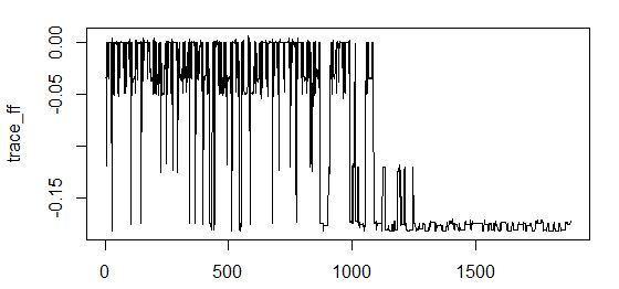
### simulated annealing search with linear model interactions stats library(scales) library(GenSA) sampleA <- bunny_dat[sample(nrow(bunny_dat), nrow(bunny_dat) / 2, replace = F), c("x", "y", "input_noise_1", "input_noise_2", "input_noise_3", "input_noise_4", "input_noise_5", "input_noise_6", "input_noise_7", "input_noise_8", "input_noise_9", "input_noise_10", "z")] sampleB <- bunny_dat[!row.names(bunny_dat) %in% rownames(sampleA), c("x", "y", "input_noise_1", "input_noise_2", "input_noise_3", "input_noise_4", "input_noise_5", "input_noise_6", "input_noise_7", "input_noise_8", "input_noise_9", "input_noise_10", "z")] #calculate parameters predictor_number <- dim(sampleA)[2] - 1 sample_size <- dim(sampleA)[1] par_v <- runif(predictor_number, min = 0, max = 1) par_low <- rep(0, times = predictor_number) par_upp <- rep(1, times = predictor_number) ############### the fitness function sa_fit_f <- function(par){ indexes <- c(1:predictor_number) for (i in 1:predictor_number){ if (par[i] >= threshold) { indexes[i] <- i } else { indexes[i] <- 0 } } local_predictor_number <- 0 for (i in 1:predictor_number){ if (indexes[i] > 0) { local_predictor_number <- local_predictor_number + 1 } } if (local_predictor_number > 0) { sampleAf <- as.data.frame(sampleA[, c(indexes[], dim(sampleA)[2])]) lm_m <- lm(formula = z ~ .^2, data = sampleAf, model = T) lm_predict <- predict(lm_m, newdata = sampleB) r_sq_validate <- 1 - sum((sampleB$z - lm_predict) ^ 2) / sum((sampleB$z - mean(sampleB$z)) ^ 2) } else { r_sq_validate <- 0 } return(-r_sq_validate) } #stimating threshold for variable inclusion threshold <- 0.5 # do it simply #run feature selection start <- Sys.time() sao <- GenSA(par = par_v, fn = sa_fit_f, lower = par_low, upper = par_upp , control = list( #maxit = 10 max.time = 300 , smooth = F , simple.function = F)) trace_ff <- data.frame(sao$trace)$function.value plot(trace_ff, type = "l") percent(- sao$value) final_vector <- c((sao$par >= threshold), T) names(sampleA)[final_vector] final_sample <- as.data.frame(sampleA[, final_vector]) Sys.time() - start # check model lm_m <- lm(formula = z ~ .^2, data = sampleA[, final_vector], model = T) summary(lm_m) What happened?
<b>[1] "5.53%"</b> > final_vector <- c((sao$par >= threshold), T) > names(sampleA)[final_vector] <b>[1] "x" "y" "input_noise_7" "input_noise_8" "input_noise_9" "z" </b> > summary(lm_m) Call: lm(formula = z ~ .^2, data = sampleA[, final_vector], model = T) Residuals: Min 1Q Median 3Q Max -0.058691 -0.023202 -0.000276 0.024953 0.050618 Coefficients: Estimate Std. Error t value Pr(>|t|) (Intercept) 0.0197777 0.0007776 25.434 <2e-16 *** <b>x -0.1547889 0.0154268 -10.034 <2e-16 *** y -0.1148349 0.0085787 -13.386 <2e-16 ***</b> input_noise_7 -0.0102894 0.0071871 -1.432 0.152 input_noise_8 -0.0013928 0.0071508 -0.195 0.846 input_noise_9 0.0026736 0.0071910 0.372 0.710 <b>x:y 1.3098676 0.1515268 8.644 <2e-16 ***</b> x:input_noise_7 0.0352997 0.0709842 0.497 0.619 x:input_noise_8 0.0653103 0.0714883 0.914 0.361 x:input_noise_9 0.0459939 0.0716704 0.642 0.521 y:input_noise_7 0.0512392 0.0710949 0.721 0.471 y:input_noise_8 0.0563148 0.0707809 0.796 0.426 y:input_noise_9 -0.0085022 0.0710267 -0.120 0.905 input_noise_7:input_noise_8 0.0129156 0.0374855 0.345 0.730 input_noise_7:input_noise_9 0.0519535 0.0376869 1.379 0.168 input_noise_8:input_noise_9 0.0128397 0.0379640 0.338 0.735 --- Signif. codes: 0 '***' 0.001 '**' 0.01 '*' 0.05 '.' 0.1 ' ' 1 Residual standard error: 0.0274 on 17957 degrees of freedom Multiple R-squared: 0.05356, Adjusted R-squared: 0.05277 F-statistic: 67.75 on 15 and 17957 DF, p-value: < 2.2e-16 We see that we miss. Noise included.
As you can see, the best value of the coefficient of determination for validation is achieved with the inclusion of noise variables. In this case, the convergence of the search algorithm is exhaustive:
Let's try to change the fitness function, save the search method.
Experiment # 6: assessing the importance of predictors using a stochastic search with a linear function of assessing importance (this is a non-greasy search in the space of inputs, the fitness function is the embedded p-values corresponding to the coefficients of the model).
We will select a set of predictors that minimize the average p-value of the coefficients in the model.
Code
# fittness based on p-values sa_fit_f2 <- function(par){ indexes <- c(1:predictor_number) for (i in 1:predictor_number){ if (par[i] >= threshold) { indexes[i] <- i } else { indexes[i] <- 0 } } local_predictor_number <- 0 for (i in 1:predictor_number){ if (indexes[i] > 0) { local_predictor_number <- local_predictor_number + 1 } } if (local_predictor_number > 0) { sampleAf <- as.data.frame(sampleA[, c(indexes[], dim(sampleA)[2])]) lm_m <- lm(formula = z ~ .^2, data = sampleAf, model = T) mean_val <- mean(summary(lm_m)$coefficients[, 4]) } else { mean_val <- 1 } return(mean_val) } #stimating threshold for variable inclusion threshold <- 0.5 # do it simply #run feature selection start <- Sys.time() sao <- GenSA(par = par_v, fn = sa_fit_f2, lower = par_low, upper = par_upp , control = list( #maxit = 10 max.time = 60 , smooth = F , simple.function = F)) trace_ff <- data.frame(sao$trace)$function.value plot(trace_ff, type = "l") percent(- sao$value) final_vector <- c((sao$par >= threshold), T) names(sampleA)[final_vector] final_sample <- as.data.frame(sampleA[, final_vector]) Sys.time() - start Result:
> percent(- sao$value) <b>[1] "-4.7e-208%"</b> > final_vector <- c((sao$par >= threshold), T) > names(sampleA)[final_vector] <b>[1] "y" "z"</b> This time everything worked out. Only original predictors were selected, since their p-values are really small.
The algorithm convergence is good in 60 seconds:
Experiment number 7: assessing the importance of predictors using a greedy search with an assessment of the importance of the quality of the trained model (this is a greedy search in the input space, the fitness function is a wrapper corresponding to the determination coefficient on the validation of the boosted decision trees model).
Code
### greedy search with wrapper GBM validation fitness library(FSelector) library(gbm) sampleA <- bunny_dat[sample(nrow(bunny_dat), nrow(bunny_dat) / 2, replace = F), c("x", "y", "input_noise_1", "input_noise_2", "input_noise_3", "input_noise_4", "input_noise_5", "input_noise_6", "input_noise_7", "input_noise_8", "input_noise_9", "input_noise_10", "z")] sampleB <- bunny_dat[!row.names(bunny_dat) %in% rownames(sampleA), c("x", "y", "input_noise_1", "input_noise_2", "input_noise_3", "input_noise_4", "input_noise_5", "input_noise_6", "input_noise_7", "input_noise_8", "input_noise_9", "input_noise_10", "z")] gbm_fit <- function(subset){ dat <- sampleA[, c(subset, "z")] gbm_fit <- gbm(formula = z ~., distribution = "gaussian", data = dat, n.trees = 50, interaction.depth = 10, n.minobsinnode = 100, shrinkage = 0.1, bag.fraction = 0.9, train.fraction = 1, n.cores = 7) gbm_predict <- predict(gbm_fit, newdata = sampleB, n.trees = 50) r_sq_validate <- 1 - sum((sampleB$z - gbm_predict) ^ 2) / sum((sampleB$z - mean(sampleB$z)) ^ 2) print(subset) print(r_sq_validate) return(r_sq_validate) } subset <- backward.search(attributes = names(sampleA)[1:(ncol(sampleA) - 1)], eval.fun = gbm_fit) subset <- forward.search(attributes = names(sampleA)[1:(ncol(sampleA) - 1)], eval.fun = gbm_fit) Result with greedy predictors:
> subset <b>[1] "x" "y"</b> > r_sq_validate <b>[1] 0.2363794</b> Got the point!
Result with the greedy exception of predictors:
> subset <b> [1] "x" "y" "input_noise_1" "input_noise_2" "input_noise_3" "input_noise_4" "input_noise_5" "input_noise_6" "input_noise_7" [10] "input_noise_9" "input_noise_10"</b> > r_sq_validate <b>[1] 0.2266737</b> It's getting worse. The inclusion of noise predictors in the model did not greatly impair the quality of the prediction on validation. And there is an explanation for this: random decision forests have a built-in regularizer and can themselves ignore non-informative inputs in the learning process.
This concludes the section of experiments on IPRs on standard methods. And in the next section, I will substantiate and show practical application, in my opinion, statistically reliable and doing a good job, based on information metrics.
3) The use of information theory for the construction of fitness functions of IPR.
The key question of this section is how to describe the concept of dependence and formulate it in the information-theoretical sense.
A source.
We need to start with the concept of informational entropy. Entropy (Shannon) is a synonym for uncertainty. The more uncertain we are about the value of a random variable, the more entropy (another synonym for information) is the realization of this value. If we consider the example of tossing a coin, then the symmetric coin of all any other variants of coins will have the greatest entropy, because we have the greatest uncertainty in the next outcome of a toss.
Formula for Shannon's entropy:
What is addiction?
Suppose we flip a coin a few times. Can we say that our uncertainty about the next outcome of the throw diminished after we saw the result of the previous throw?
Suppose we have a coin that lands with an eagle with a probability of 2/3 after falling heads, and vice versa - after falling of an eagle, it lands on heads with a probability of 2/3. At the same time, the unconditional frequency of the fallouts of the eagle and tails remains 50/50.
For such a coin after a falling eagle, the frequency of tails is no longer 1/2, and vice versa. So, our uncertainty about the next outcome of the throw has decreased (we don’t expect 50/50).
To understand the phenomenon of dependence, we recall that probability theory defines independence as follows:
p (x, y) == p (x) * p (y)
thus, the probability of the joint realization of events is equal to the product of the probabilities of their own realizations.
If this is observed, the events are independent in a mathematical sense. If
p (x, y)! = p (x) * p (y)
then events are not mathematically independent.
The same principle underlies the formula for measuring the relationship between two (and more) random variables in information theory.
We emphasize that here dependence is understood in a probabilistic sense. The analysis of causality requires a more comprehensive review, including both the analysis of false correlations and redundancy (through the use of mutual information), and the involvement of expert knowledge about the object under study.
Mutual Information
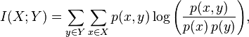
You can also output mutual information through entropies:
In simple words, mutual information is the amount of entropy (uncertainty) that leaves the system, if there is a predictive variable (or several variables). For example, the entropy of a random variable is 3 bits. Mutual information is 2 bits. Hence, by 2/3, the uncertainty about the implementation of a random variable is compensated by the presence of a predictor.
Mutual information has the following properties:
- symmetry
- can be defined for discrete and continuous variables
- vanishes if X and Y are independent
- the normalized measure of mutual information takes the value 1 if the two variables completely determine each other
Mutual information satisfies some of the requirements for the ideal measure of dependence, formulated in:
Granger, C, E. Maasoumi e J. Racine, 'A Dependence Metric for Possibly Nonlinear Processes', Journal of Time Series Analysis 25, 2004, 649-669.
There is one property of mutual information ( VI ) that is useful to know when applying this measure:
- A CI can reach its maximum equal to the smaller of the entropy values for entry and exit (predictor and dependent variable).
This means that if our input variable has an entropy of 10 bits, and the output variable has 3 bits, then the maximum information that the input variable can transmit to the output is 3 bits. This is the maximum VI, which can be in such a system.
Another option is that the input variable has an entropy of 3 bits, and the output is 10 bits. The maximum information that an input can carry to the output is 3 bits, and this is the possible maximum of the VI.
If the VI value is divided by the entropy of the dependent variable, we get a value in the range [0, 1], which, by analogy with the correlation coefficient, indicates how, without taking into account the scale of values, the input variable determines the dependent variable.
There are a number of arguments for using VIs, although it involves a number of tradeoffs:
- The method allows to find dependencies of an arbitrary type (linear and non-linear) in a space of arbitrary dimension;
- The method will exclude all input variables if their total or individual information content is lower than the statistically significant one;
- The weak side of the method is the fact that weak dependencies - which barely exceed the level of statistical noise - will be hidden from the eyes of the researcher after applying the numerically calculated quantile of the VI metric;
- With a small number of significant discrete input variables, the researcher is able to build a human-readable set of rules that allow interpretation of the dependencies found;
- It is not necessary to compose randomized committees of models (by analogy with random forest and busting machines), since the method in itself tries many possible levels of "tree depth" for all the selected predictors and returns the most significant, in a statistical sense, combination of informative features;
- The method is very expensive, especially in comparison with other methods combining greedy gradient descent and a simpler fitness function that does not require simulation corrections;
- , , , .
.
, , . , , , .
— (Multiinformation) (Total Correlation).
A source:
:
:
Watanabe S (1960). Information theoretical analysis of multivariate correlation, IBM Journal of Research and Development 4, 66–82
( ) , . , ( 1 n) ( 1 m), . , - .
, .
, , . :
- 1) . , — , , , — . , , 2. , , .
- 2) . , , . , , , — .
- 3) . , .
.
, , :
, . . , . ., , 1973 — 512 .
.. — « ».
, .
, , , , .
, n N.
. , .
100 .
1000 .
, , .
, , . , . .:
1.
2.
, , . . , ( ). , .
, .
. . , , . .
( ), .
. . , , , . , 1 000 51% , - . . .
- .
- ) .
- ) , , , ( ) « » .
- ) numeric , [0, 1] (0) (1) — SA.
- ) , , -, .
- ) - ; (, 0.9) .
- ) . , .
- ) , .
«» . — , :
optim_var_num < — log(x = sample_size / 100, base = round(mean_levels, 0))
, , , , , n , n 100. , , , .
, , .
, , ( ), :
threshold < — 1 — optim_var_num / predictor_number
, . .
, : , .
17 973 , 12 , 5 . , 3,226.
, 0,731.
?
3 . , 5 ^ 3,226 178 , 100 .
.
№8 , () ( , - — ).
0,9 ( ) 10 -, 1 1 ( ). 10 .
Code
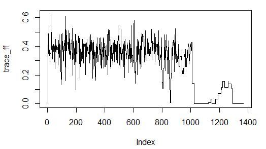
############## simlated annelaing search with mutual information fitness function library(infotheo) # measured in nats, converted to bits library(scales) library(GenSA) sampleA <- bunny_dat[sample(nrow(bunny_dat), nrow(bunny_dat) / 2, replace = F), c("x", "y", "input_noise_1", "input_noise_2", "input_noise_3", "input_noise_4", "input_noise_5", "input_noise_6", "input_noise_7", "input_noise_8", "input_noise_9", "input_noise_10", "z")] sampleB <- bunny_dat[!row.names(bunny_dat) %in% rownames(sampleA), c("x", "y", "input_noise_1", "input_noise_2", "input_noise_3", "input_noise_4", "input_noise_5", "input_noise_6", "input_noise_7", "input_noise_8", "input_noise_9", "input_noise_10", "z")] # discretize all variables dat <- sampleA disc_levels <- 5 for (i in 1:13){ naming <- paste(names(dat[i]), 'discrete', sep = "_") dat[, eval(naming)] <- discretize(dat[, eval(names(dat[i]))], disc = "equalfreq", nbins = disc_levels)[,1] } sampleA <- dat[, 14:26] #calculate parameters predictor_number <- dim(sampleA)[2] - 1 sample_size <- dim(sampleA)[1] par_v <- runif(predictor_number, min = 0, max = 1) par_low <- rep(0, times = predictor_number) par_upp <- rep(1, times = predictor_number) #load functions to memory shuffle_f_inp <- function(x = data.frame(), iterations_inp, quantile_val_inp){ mutins <- c(1:iterations_inp) for (count in 1:iterations_inp){ xx <- data.frame(1:dim(x)[1]) for (count1 in 1:(dim(x)[2] - 1)){ y <- as.data.frame(x[, count1]) y$count <- sample(1 : dim(x)[1], dim(x)[1], replace = F) y <- y[order(y$count), ] xx <- cbind(xx, y[, 1]) } mutins[count] <- multiinformation(xx[, 2:dim(xx)[2]]) } quantile(mutins, probs = quantile_val_inp) } shuffle_f <- function(x = data.frame(), iterations, quantile_val){ height <- dim(x)[1] mutins <- c(1:iterations) for (count in 1:iterations){ x$count <- sample(1 : height, height, replace = F) y <- as.data.frame(c(x[dim(x)[2] - 1], x[dim(x)[2]])) y <- y[order(y$count), ] x[dim(x)[2]] <- NULL x[dim(x)[2]] <- NULL x$dep <- y[, 1] rm(y) receiver_entropy <- entropy(x[, dim(x)[2]]) received_inf <- mutinformation(x[, 1 : dim(x)[2] - 1], x[, dim(x)[2]]) corr_ff <- received_inf / receiver_entropy mutins[count] <- corr_ff } quantile(mutins, probs = quantile_val) } ############### the fitness function fitness_f <- function(par){ indexes <- c(1:predictor_number) for (i in 1:predictor_number){ if (par[i] >= threshold) { indexes[i] <- i } else { indexes[i] <- 0 } } local_predictor_number <- 0 for (i in 1:predictor_number){ if (indexes[i] > 0) { local_predictor_number <- local_predictor_number + 1 } } if (local_predictor_number > 1) { sampleAf <- as.data.frame(sampleA[, c(indexes[], dim(sampleA)[2])]) pred_entrs <- c(1:local_predictor_number) for (count in 1:local_predictor_number){ pred_entrs[count] <- entropy(sampleAf[count]) } max_pred_ent <- sum(pred_entrs) - max(pred_entrs) pred_multiinf <- multiinformation(sampleAf[, 1:dim(sampleAf)[2] - 1]) pred_multiinf <- pred_multiinf - shuffle_f_inp(sampleAf, iterations_inp, quantile_val_inp) if (pred_multiinf < 0){ pred_multiinf <- 0 } pred_mult_perc <- pred_multiinf / max_pred_ent inf_corr_val <- shuffle_f(sampleAf, iterations, quantile_val) receiver_entropy <- entropy(sampleAf[, dim(sampleAf)[2]]) received_inf <- mutinformation(sampleAf[, 1:local_predictor_number], sampleAf[, dim(sampleAf)[2]]) if (inf_corr_val - (received_inf / receiver_entropy) < 0){ fact_ff <- (inf_corr_val - (received_inf / receiver_entropy)) * (1 - pred_mult_perc) } else { fact_ff <- inf_corr_val - (received_inf / receiver_entropy) } } else if (local_predictor_number == 1) { sampleAf<- as.data.frame(sampleA[, c(indexes[], dim(sampleA)[2])]) inf_corr_val <- shuffle_f(sampleAf, iterations, quantile_val) receiver_entropy <- entropy(sampleAf[, dim(sampleAf)[2]]) received_inf <- mutinformation(sampleAf[, 1:local_predictor_number], sampleAf[, dim(sampleAf)[2]]) fact_ff <- inf_corr_val - (received_inf / receiver_entropy) } else { fact_ff <- 0 } return(fact_ff) } ########## estimating threshold for variable inclusion iterations = 10 quantile_val = 0.9 iterations_inp = 1 quantile_val_inp = 1 levels_arr <- numeric() for (i in 1:predictor_number){ levels_arr[i] <- length(unique(sampleA[, i])) } mean_levels <- mean(levels_arr) optim_var_num <- log(x = sample_size / 100, base = round(mean_levels, 0)) if (optim_var_num / predictor_number < 1){ threshold <- 1 - optim_var_num / predictor_number } else { threshold <- 0.5 } #run feature selection start <- Sys.time() sao <- GenSA(par = par_v, fn = fitness_f, lower = par_low, upper = par_upp , control = list( #maxit = 10 max.time = 300 , smooth = F , simple.function = F)) trace_ff <- data.frame(sao$trace)$function.value plot(trace_ff, type = "l") percent(- sao$value) final_vector <- c((sao$par >= threshold), T) names(sampleA)[final_vector] final_sample <- as.data.frame(sampleA[, final_vector]) Sys.time() - start Result:
> percent(- sao$value) <b>[1] "18.1%"</b> > final_vector <- c((sao$par >= threshold), T) > names(sampleA)[final_vector] <b>[1] "x_discrete" "y_discrete" "input_noise_2_discrete" "z_discrete" </b> > final_sample <- as.data.frame(sampleA[, final_vector]) > > Sys.time() - start Time difference of 10.00453 mins . . — .
20 , - 1 .
Result:
> percent(- sao$value) <b><b>[1] "18.2%"</b></b> > final_vector <- c((sao$par >= threshold), T) > names(sampleA)[final_vector] <b><b>[1] "x_discrete" "y_discrete" "input_noise_1_discrete" </b>"z_discrete" </b> > final_sample <- as.data.frame(sampleA[, final_vector]) > > Sys.time() - start Time difference of 20.00585 mins — .
18% . .
( ):
Minimum-redundancy-maximum-relevance (mRMR)
. :
«Feature selection based on mutual information: criteria of max-dependency, max-relevance, and min-redundancy,»
Hanchuan Peng, Fuhui Long, and Chris Ding
IEEE Transactions on Pattern Analysis and Machine Intelligence,
Vol. 27, No. 8, pp.1226-1238, 2005
, ( ) . .
() , () .
() , , , . , .
() , . , ( ).
, , , , , ( ) , . , mRMR , .
() , — limited sampling bias.
mRMR . , , , , .
.
, , GBM, p-values .
, . , , , . , XY-Noise1 . , ( ), Align Technology. , , , Gradient Boosted Trees ( . ).
, , , . , , , , .
, , . . , , .
. , , , , . , .
github: Git
:
- Greedy Function Approximation: A Gradient Boosting Machine by J. Friedman
- , . . , . ., , 1973 — 512 .
- .. — « ».
- Analytical estimates of limited sampling biases in different information measures by S. Panzeri at.al.
- Estimation of Entropy and Mutual Information by L. Paninski
- Entropy-Based Independence Test by A. Dionísio at.al.
- , , DJI, .
- Measuring dependence powerfully and equitably by Y. Reshef et.al.
- «Feature selection based on mutual information: criteria of max-dependency, max-relevance, and min-redundancy,» Hanchuan Peng, Fuhui Long, and Chris Ding IEEE Transactions on Pattern Analysis and Machine Intelligence, Vol. 27, No. 8, pp.1226-1238, 2005
- Watanabe S (1960). Information theoretical analysis of multivariate correlation, IBM Journal of Research and Development 4, 66–82
- Gradient boosting machines, a tutorial.
- Claude E. Shannon, Warren Weaver. The Mathematical Theory of Communication. Univ of Illinois Press, 1949
Source: https://habr.com/ru/post/303750/
All Articles