Connect MATLAB to Wolfram Mathematica

Calling MATLAB from Mathematica with MATLink

How can you call MATLAB functions directly from Mathematica and organize the exchange of data and variables between the two systems?

To do this, there is a cross-platform package called MATLink . With it, it is easy to organize a call to the MATLAB functions directly from Mathematica and transfer various data from one system to another.

I will give a small instruction:
')
● Installation
First, go to the main page of MATLink and follow the instructions there. The easiest way is to download the archive and unpack it into this folder:

In [1]: =

SystemOpen@FileNameJoin[{$UserBaseDirectory, "Applications"}] 

Next, follow the instructions for the specific operating system in the “Link with MATLAB” section of the main page.

● Using MATLink

MATLink can be downloaded by calculating a cell with the code:

In [2]: =

 Needs["MATLink`"] 

And then start MATLAB with the command:

In [3]: =

 OpenMATLAB [] 

This will launch a new process in MATLAB, with which Mathematica can interact.

To use arbitrary MATLAB commands, use MEvaluate . The data will be transmitted as a string.

Example:

In [4]: ​​=

 MEvaluate["magic(4)"] 

Out [4] =

 (* ==> ans = 16 2 3 13 5 11 10 8 9 7 6 12 4 14 15 1 *) 

To transfer data to MATLAB, you must use MSet :

In [5]: =

 MSet["x", Range[10]];MEvaluate["x"] 

Out [5] =

 (* ==> x = 1 2 3 4 5 6 7 8 9 10 *) 

To get data back, follow MGet's use:

In [6]: =

 MGet["x"] 

Out [6] =

 (* ==> {1., 2., 3., 4., 5., 6., 7., 8., 9., 10.} *) 

A large number of data types are supported, including sparse arrays, structures, and cells.

MATLAB functions can be called directly from Mathematica using the MFunction function:

In [7]: =

 eig = MFunction["eig"]; eig[{{1, 2}, {3, 1}}] 

Out [7] =

 (* ==> {{3.44949}, {-1.44949}} *) 

In the documentation you can read more about the features of use and other functionalities.

Some simple examples

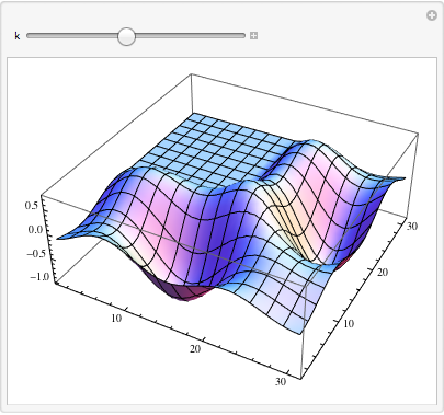
Let's build in Mathematica for the beginning the surface of the MATLAB logo and add a manipulator that will regulate the oscillation period:

In [8]: =

 Manipulate[ ListPlot3D@MFunction["membrane"][k], {k, 1, 12, 1} ] 

Out [8] =


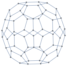
Fullerene structure (bucky ball) straight from MATLAB:

In [9]: =

 AdjacencyGraph@Round@MFunction["bucky"][] 

Out [9] =


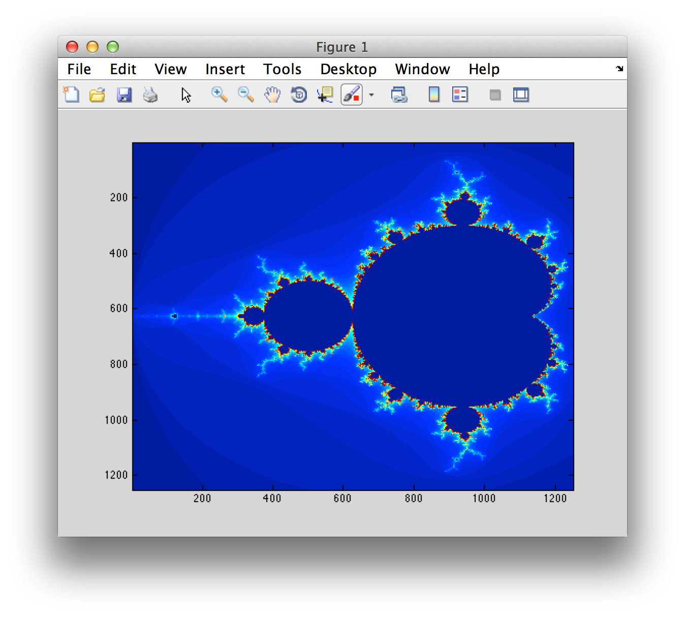
Displaying data from Mathematica in a separate scalable window for images that are used in MATLAB is also easy:

In [9]: =

 mlf = LibraryFunctionLoad["demo_numerical", "mandelbrot", {Complex}, Integer]; mandel = Table[mlf[x + I y], {y, -1.25, 1.25, .002}, {x, -2., 0.5, .002}]; MFunction["image", "Output" -> False][mandel] 

Out [9] =

Some examples are more complicated.

The following examples illustrate real-world solutions using MATLink, allowing you to use the best qualities of MATLAB and Mathematica.

● Fast Delaunay Triangulations

Mathematica contains the DelaunayTriangulation function inside the ComputationalGeometry package (in the 10th version, this package was built into the kernel and now this function is named DelaunayMesh , it is optimized and now its performance is not inferior to MATLAB - ed.) , But it works very slowly (although she has her own strengths, such as using exact arithmetic and working with collinear points). This, in turn, leads to the fact that ListDensityPlot works very inefficiently (which becomes noticeable when building several thousand points or more). Using MATLink, we can use the Delone function from MATLAB to calculate the Delaunay triangulation of a certain set of points as follows:

In [10]: =

 delaunay = Composition[Round, MFunction["delaunay"]]; 

Since the Mathematica function returns a list of adjacent vertices, we need to post-process the result in order to compare it with the result from MATLAB:

In [11]: =

 Needs["ComputationalGeometry`"]; delaunayMma[points_] := Module[{tr, triples}, tr = DelaunayTriangulation[points]; triples = Flatten[ Function[{v, list}, Switch[Length[list], (* account for nodes with connectivity 2 or less *) 1, {}, 2, {Flatten[{v, list}]}, _, {v, ##}& @@@ Partition[list, 2, 1, {1, 1}]] ] @@@ tr, 1]; Cases[GatherBy[triples, Sort], a_ /; Length[a] == 3 :> a[[1]]] ] 

A random set of points usually has a unique Delaunay triangulation, so we will need to check that the systems produce the same result.

In [12]: =

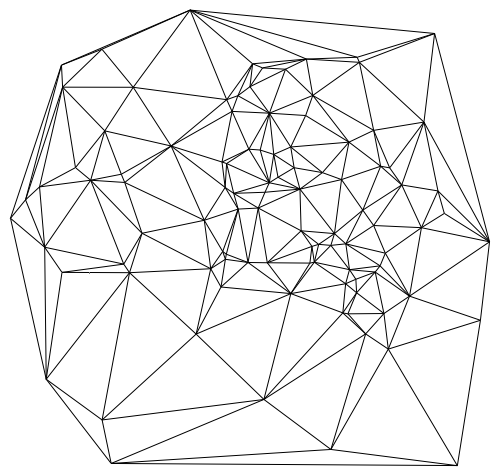
 pts = RandomVariate[NormalDistribution[], {100, 2}]; Sort[Sort /@ delaunay[pts]] === Sort[Sort /@ delaunayMma[pts]] 

And build triangulation using:

In [13]: =

 trianglesToLines[t_] := Union@Flatten[{{#1, #2}, {#2, #3}, {#1, #3}} & @@ Transpose[Sort /@ t], {{1, 3}, {2}}]; Graphics@GraphicsComplex[pts, Line@trianglesToLines@delaunay[pts]] 

Out [13]: =


However, besides the fact that delaunay works much faster than the DelaunayTriangulation (especially for large data sets), it is also faster than the triangulator , which is used inside ListDensityPlot . Therefore, we can use delaunay from MATLAB to develop our version of listDensityPlot , which works faster than the built-in function, and can also process large data sets as follows:

In [14]: =

 Options[listDensityPlot] = Options[Graphics] ~Join~ {ColorFunction -> Automatic, MeshStyle -> None, Frame -> True}; listDensityPlot[data_?MatrixQ, opt : OptionsPattern[]] := Module[{in, out, tri, colfun}, tri = delaunay[data[[All, 1;;2]]]; colfun = OptionValue[ColorFunction]; If[Not@MatchQ[colfun, _Symbol | _Function], Check[colfun = ColorData[colfun], colfun = Automatic]]; If[colfun === Automatic, colfun = ColorData["LakeColors"]]; Graphics[ GraphicsComplex[data[[All, 1;;2]], GraphicsGroup[{EdgeForm[OptionValue[MeshStyle]], Polygon[tri]}], VertexColors -> colfun /@ Rescale[data[[All, 3]]] ], Sequence @@ FilterRules[{opt}, Options[Graphics]], Method -> {"GridLinesInFront" -> True} ] ] 

Let's now compare our function with the built-in function, using an array of 30,000 points:

In [15]: =

 pts = RandomReal[{-1, 1}, {30000, 2}]; values = Sin[3 Sqrt[#1^2 + #2^2]] & @@@ pts; 

In [16]: =

 listDensityPlot[ArrayFlatten[{{pts, List /@ values}}], Frame -> True] // AbsoluteTiming 

Out [16] =

 {0.409001, --Graphics--} 

In [17]: =

 ListDensityPlot[ArrayFlatten[{{pts, List /@ values}}]] // AbsoluteTiming 

Out [17] =

 {12.416587, --Graphics--} 

The difference in execution speed turned out to be quite significant (~ 30 times). ListDensityPlot is practically unusable for working with hundreds of thousands of points, while the listDensityPlot only takes a few seconds.

It is also important to note that for measuring the speed of MATLink, you must use the AbsoluteTiming function, which calculates all elapsed time, while Timing measures only the time when the CPU was used by the Mathematica core, not measuring the time that MATLAB spent.

● Filtering audio data using signal processing tools

As you know, signal processing functionality was missing in Mathematica until version 9, and is still inferior to MATLAB tools in terms of functionality and ease of use. Suppose we have version 8 of Mathematica, there are no new functions, and we want to conduct a frequency analysis of some audio file and implement filtering. Here's how to do it:

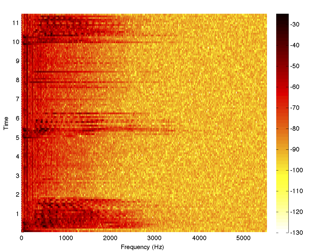
In [18]: =

 {data, fs} = {#[[1, 1, 1]], #[[1, 2]]} &@ExampleData[{"Sound", "Apollo13Problem"}]; spectrogram = MFunction["spectrogram", "Output" -> False]; (* Use MATLAB's spectrogram *) spectrogram[data, 1000, 0, 1024, fs] 

Obviously, the frequencies mainly fall in the range below 2.5 kHz, so we can develop a low-pass filter in MATLAB, as well as make an auxiliary function that will return the filtered data:

In [19]: =

 MSet["fs", fs]; MEvaluate[" [z, p, k] = butter(6, 2.5e3/fs, 'low') ; [sos, g] = zp2sos(z, p, k) ; Hd = dfilt.df2tsos(sos, g) ; "] filter = MFunction["myfilt", "@(x)filter(Hd,x)"]; 

Out [19] =


Now we have prepared everything to apply the filter function to the data directly from Mathematica. This example shows how we can fill in the gaps in functionality. Thus, we can save a large amount of time to design a filter in Mathematica (and this is not the easiest task) and many hours to debug it. The code for the Butterworth filter can be taken from anywhere - from file sharing or Stack Overflow, from fragments of previously written code, or, as in this case, from the example in the documentation. Small changes in parameters for current needs, and we can now work with this material in Mathematica.

As a final example, I propose to process some data using our filter and build a spectrogram:

In [19]: =

 filteredData = filter@data; spectrogram[filteredData, 1000, 0, 1024, fs] 

Purely for fun, we can play both audio files - filtered and source — and compare the difference in their sound:

In [20]: =

 ListPlay[data, SampleRate -> fs] ListPlay[filteredData, SampleRate -> fs]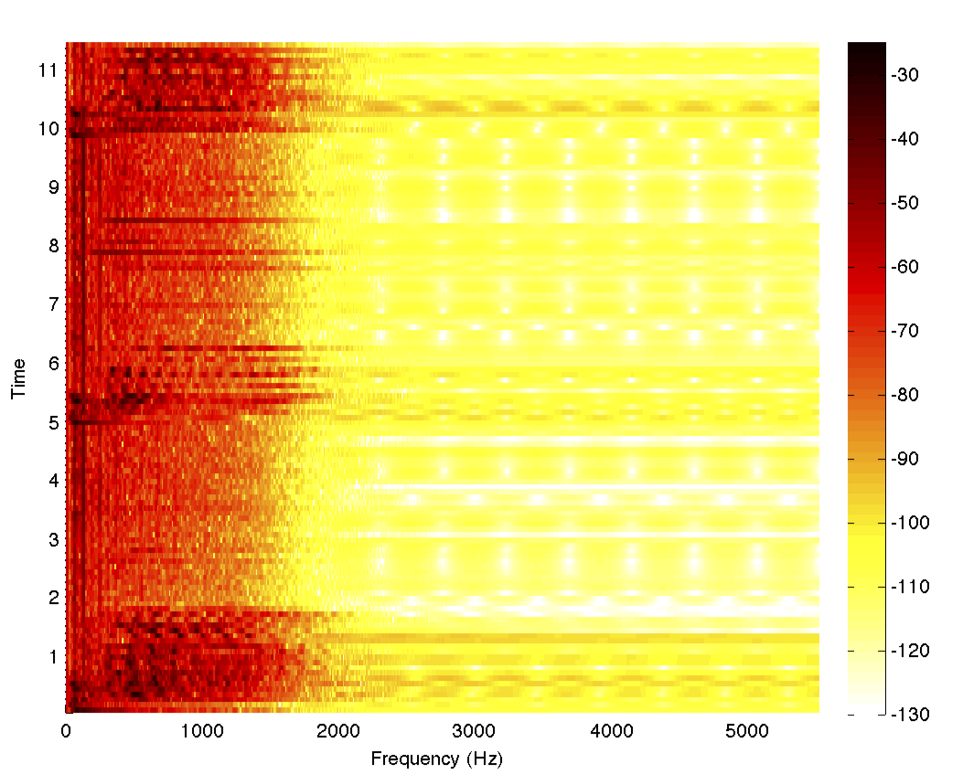 

If suddenly you find any errors and problems in the work of MATLink, please report them to the post office (matlink.m@gmail.com), either on GitHub, or in the comments to the original of this article .

Additions

● Calling MATLAB from Mathematica using NETLink

A quick note about how you can invoke MATLAB using NETLink in the Windows operating system using the MATLAB COM interface:

In [21]: =

 Needs["NETLink`"] matlab = CreateCOMObject["matlab.application"] 

Out [21] =

 «NETObject[COMInterface[MLApp.DIMLApp]]» 

Now you can access the MATLAB functions:

In [22]: =

 In[4]:= matlab@Execute["version"] 

Out [22] =

 " ans = 7.9.0.529 (R2009b) " 

In [23]: =

 matlab@Execute["a=2"];matlab@Execute["a*2"] 

Out [23] =

 " ans = 4 " 

● About converting expressions from Mathematica syntax to MATLAB syntax

There is a package called ToMatlab that converts expressions from Mathematica to their MATLAB equivalents. Here is an example:

In [24]: =

 <<ToMatlab` Expand[(x + Log@y)^5] // ToMatlab 

Out [24]: =

 x.^5+5.*x.^4.*log(y)+10.*x.^3.*log(y).^2+10.*x.^2.*log(y).^3+5.* ... x.*log(y).^4+log(y).^5; 

You may notice that expressions are quite conveniently broken using ...;

Here is another example with matrix conversion:

In [25]: =

 RandomInteger[5, {5, 5}] // ToMatlab 

Out [25]: =

 [5,0,5,3,4; 5,5,3,0,2; 1,4,4,4,4; 0,3,2,5,5; 4,5,5,1,1]; 

It is worth noting that such things as general definitions cannot be converted to MATLAB syntax. Of course, those constructions that are not supported by MATLAB — template expressions, for example, cannot be converted either.

To install this package, simply extract the ToMatlab.m file to the folder:

In [26]: =

 FileNameJoin[{$UserBaseDirectory, "Applications"}] 

For questions about Wolfram technologies, write to info-russia@wolfram.com