OpenGL ES 2.0. One million particles

In this article we will look at one of the options for implementing the particle system on OpenGL ES 2.0. Let's talk in detail about the limitations, we will describe the principles and analyze a small example.

Restrictions

In general, we will require two additional properties from OpenGL ES 2.0 (the specification does not require their presence):

• Vertex Texture Fetch . Allows us to access texture maps via texture units from the vertex shader. You can request the maximum number of units supported by the graphics processor using the glGetIntegerv function with the parameter name GL_MAX_VERTEX_TEXTURE_IMAGE_UNITS. The table below presents data on the currently popular processors.
• Fragment high floating-point precision . Allows us to perform calculations with high accuracy in a fragment shader. You can request the accuracy and range of values ​​using the glGetShaderPrecisionFormat function with the GL_FRAGMENT_SHADER and GL_HIGH_FLOAT parameter names for the shader type and data type, respectively. For all the processors listed in the table, the accuracy is 23 bits with a range of values ​​from -2 ^ 127 to 2 ^ 127, with the exception of Snapdragon Andreno 2xx , for this series the range is from -2 ^ 62 to 2 ^ 62.

')
Processor Information:

CPU	Vertex TIU	Accuracy	Range
Snapdragon Adreno 2xx	four	23	[-2 ^ 62, 2 ^ 62]
Snapdragon Adreno 3xx	sixteen	23	[-2 ^ 127, 2 ^ 127]
Snapdragon Adreno 4xx	sixteen	23	[-2 ^ 127, 2 ^ 127]
Snapdragon Adreno 5xx	sixteen	23	[-2 ^ 127, 2 ^ 127]
Intel HD Graphics	sixteen	23	[-2 ^ 127, 2 ^ 127]
ARM Mali-T6xx	sixteen	23	[-2 ^ 127, 2 ^ 127]
ARM Mali-T7xx	sixteen	23	[-2 ^ 127, 2 ^ 127]
ARM Mali-T8xx	sixteen	23	[-2 ^ 127, 2 ^ 127]
NVIDIA Tegra 2/3/4	0	0	0
NVIDIA Tegra K1 / X1	32	23	[-2 ^ 127, 2 ^ 127]
PowerVR SGX (Series5)	eight	23	[-2 ^ 127, 2 ^ 127]
PowerVR SGX (Series5XT)	eight	23	[-2 ^ 127, 2 ^ 127]
PowerVR Rogue (Series6)	sixteen	23	[-2 ^ 127, 2 ^ 127]
PowerVR Rogue (Series6XT)	sixteen	23	[-2 ^ 127, 2 ^ 127]
VideoCore IV	eight	23	[-2 ^ 127, 2 ^ 127]
Vivante GC1000	four	23	[-2 ^ 127, 2 ^ 127]
Vivante GC4000	sixteen	23	[-2 ^ 127, 2 ^ 127]

There is a problem with NVIDIA Tegra 2/3/4 , a number of popular devices such as the Nexus 7, HTC One X, ASUS Transformer work on this series.

Particle system

Considering the systems of particles generated on the CPU, in the context of increasing the amount of data being processed (the number of particles), the main performance problem is copying (uploading) data from the RAM to the video memory on each frame. Therefore, our main task is to avoid this copying, transferring the calculations to the non-operational mode on the graphics processor.

Recall that in OpenGL ES 2.0 there are no built-in mechanisms such as Transform Feedback (available in OpenGL ES 3.0) or Compute Shader (available in OpenGL ES 3.1), allowing you to perform calculations on the GPU.

The essence of the method is to use as a buffer data for storage, characterizing a particle, values ​​(coordinates, accelerations, etc.) - textures and process them with vertex and fragment shaders. Also, as we store and load the normals, talking about the Normal mapping . The size of the buffer, in our case, is proportional to the number of particles to be processed. Each texel stores a separate value (quantities, if there are several) for an individual particle. Accordingly, the number of processed quantities is inversely related to the number of particles. For example, in order to process positions and accelerations for 1048576 particles, we need two textures of 1024x1024 (if there is no need to preserve the aspect ratio)

There are additional restrictions that we need to take into account. To be able to record any information, the format of the pixel texture data must be supported by the implementation as a color-renderable format . This means that we can use the texture as a color buffer in the frame -by- frame rendering . The specification describes only three such formats: GL_RGBA4, GL_RGB5_A1, GL_RGB565 . Considering the subject area, we need at least 32 bits per pixel to process values ​​such as coordinates or accelerations (for the two-dimensional case). Therefore, the formats mentioned above are not enough for us.

To ensure the necessary minimum, we consider two additional types of textures: GL_RGBA8 and GL_RGBA16F . Such textures are often called LDR (SDR) and HDR textures, respectively.

• GL_RGBA8 is supported by the specification, we can load and read textures with this format. For recording, we need to require the extension OES_rgb8_rgba8 .
  
• GL_RGBA16F is not supported by the specification, in order to load and read textures with this format, we need the extension GL_OES_texture_half_float . Moreover, in order to obtain an acceptable quality result, we need the support of linear filters for minification and magnification of such textures. The extension GL_OES_texture_half_float_linear is responsible for this . For recording, we need the extension GL_EXT_color_buffer_half_float .

According to GPUINFO for 2013 - 2015, support for extensions is as follows:

Expansion	Devices (%)
OES_rgb8_rgba8	98.69%
GL_OES_texture_half_float	61.5%
GL_OES_texture_half_float_linear	43.86%
GL_EXT_color_buffer_half_float	32.78%

Generally speaking, HDR textures are more suitable for our purposes. First, they allow us to process more information without compromising performance, for example, to manipulate particles in three-dimensional space without increasing the number of buffers. Secondly, there is no need for intermediate mechanisms for unpacking and packing data when reading and writing, respectively. But, due to poor support for HDR textures, we will choose LDR.

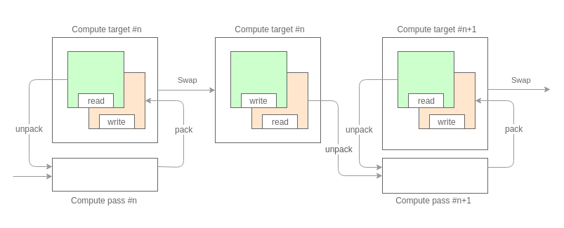
So, going back to the point, the general scheme of what we are going to do looks like this:



The first thing we need is to split the calculations into passes. The splitting depends on the number and type of characterizing values ​​that we are going to work on. Based on the fact that we have a texture as a data buffer and taking into account the limitations on the format of pixel data described above, each pass can process no more than 32 bits of information on each particle. For example, on the first pass, we calculated the accelerations (32 bits, 16 bits per component), on the second, the positions were updated (32 bits, 16 bits per component).

Each pass processes data in double buffering mode. This provides access to the system state of the previous frame.

The core of the aisle is the usual texture mapping into two triangles, where our data buffers act as texture maps. The general view of shaders is as follows:

//   attribute vec2 a_vertex_xy; attribute vec2 a_vertex_uv; varying vec2 v_uv; void main() { gl_Position = vec4(a_vertex_xy, 0.0, 1.0); v_uv = a_vertex_uv; } 

 //   precision highp float; varying vec2 v_uv; //    // ( ) uniform sampler2D u_prev_state; //     // ( ) uniform sampler2D u_pass_0; ... uniform sampler2D u_pass_n; //   <type> unpack(vec4 raw); <type_0> unpack_0(vec4 raw); ... <type_n> unpack_1(vec4 raw) //   vec4 pack(<type> data); void main() { //      //     v_uv <type> data = unpack(texture2D(u_prev_state, v_uv)); <type_0> data_pass_0 = unpack_0(texture2D(u_pass_0, v_uv)); ... <type_n> data_pass_n = unpack_n(texture2D(u_pass_n, v_uv)); //   <type> result = ... //     gl_FragColor = pack(result); } 

The implementation of the unpacking / packing functions depends on the quantities that we process. At this stage, we rely on the requirement, described at the beginning, of high precision calculations.
For example, for two-dimensional coordinates (components [x, y] of 16 bits), the functions might look like this:

 vec4 pack(vec2 value) { vec2 shift = vec2(255.0, 1.0); vec2 mask = vec2(0.0, 1.0 / 255.0); vec4 result = fract(value.xxyy * shift.xyxy); return result - result.xxzz * mask.xyxy; } vec2 unpack(vec4 value) { vec2 shift = vec2(1.0 / 255.0, 1.0); return vec2(dot(value.xy, shift), dot(value.zw, shift)); } 

Drawing

After the computation stage, the rendering phase follows. To access the particles at this stage, we need, for sorting, some external index. The vertex buffer ( Vertex Buffer Object ) with the texture coordinates of the data buffer will act as such an index. The index is created and initialized (unloaded into the memory of the video device) once and does not change in the process.

In this step, the requirement for access to texture maps takes effect. The vertex shader is similar to the fragment shader from the calculation stage:

 //   //   attribute vec2 a_data_uv; //  ,   uniform sampler2D u_positions; //   ( ) uniform sampler2D u_data_0; ... uniform sampler2D u_data_n; //    vec2 unpack(vec4 data); //     <type_0> unpack_0(vec4 data); ... <type_n> unpack_n(vec4 data); void main() { //      vec2 position = unpack(texture2D(u_positions, a_data_uv)); gl_Position = vec4(position * 2.0 - 1.0, 0.0, 1.0); //      <type_0> data_0 = unpack(texture2D(u_data_0, a_data_uv)); ... <type_n> data_n = unpack(texture2D(u_data_n, a_data_uv)); } 

Example

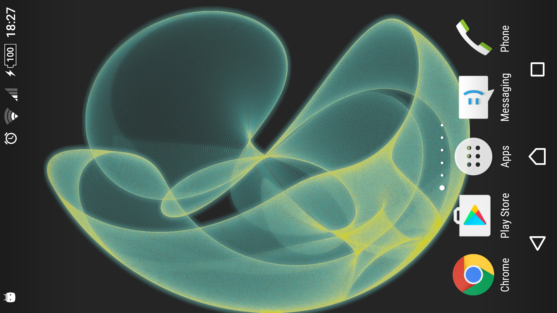
As a small example, we will try to generate a dynamic system of 1048576 particles, known as Strange Attractor .



Frame processing consists of several stages:

Compute stack

At the computation stage, we will have only one independent pass, which is responsible for the positioning of the particles. It is based on a simple formula:

  Xn+1 = sin(a * Yn) - cos(b * Xn) Yn+1 = sin(c * Xn) - cos(d * Yn) 

Such a system is also called Peter de Jong Attractors . Over time, we will change only the coefficients.

 //   attribute vec2 a_vertex_xy; varying vec2 v_uv; void main() { gl_Position = vec4(a_vertex_xy, 0.0, 1.0); v_uv = a_vertex_xy * 0.5 + 0.5; } 

 //   precision highp float; varying vec2 v_uv; uniform lowp float u_attractor_a; uniform lowp float u_attractor_b; uniform lowp float u_attractor_c; uniform lowp float u_attractor_d; vec4 pack(vec2 value) { vec2 shift = vec2(255.0, 1.0); vec2 mask = vec2(0.0, 1.0 / 255.0); vec4 result = fract(value.xxyy * shift.xyxy); return result - result.xxzz * mask.xyxy; } void main() { vec2 pos = v_uv * 4.0 - 2.0; for(int i = 0; i < 3; ++i) { pos = vec2(sin(u_attractor_a * pos.y) - cos(u_attractor_b * pos.x), sin(u_attractor_c * pos.x) - cos(u_attractor_d * pos.y)); } pos = clamp(pos, vec2(-2.0), vec2(2.0)); gl_FragColor = pack(pos * 0.25 + 0.5); } 

Renderer Stage

At the stage rendering stage, we will render our particles with ordinary sprites.

 //   //  attribute vec2 a_positions_uv; //  (,    ) uniform sampler2D u_positions; varying vec4 v_color; vec2 unpack(vec4 value) { vec2 shift = vec2(0.00392156863, 1.0); return vec2(dot(value.xy, shift), dot(value.zw, shift)); } void main() { vec2 position = unpack(texture2D(u_positions, a_positions_uv)); gl_Position = vec4(position * 2.0 - 1.0, 0.0, 1.0); v_color = vec4(0.8); } 

 //   precision lowp float; varying vec4 v_color; void main() { gl_FragColor = v_color; }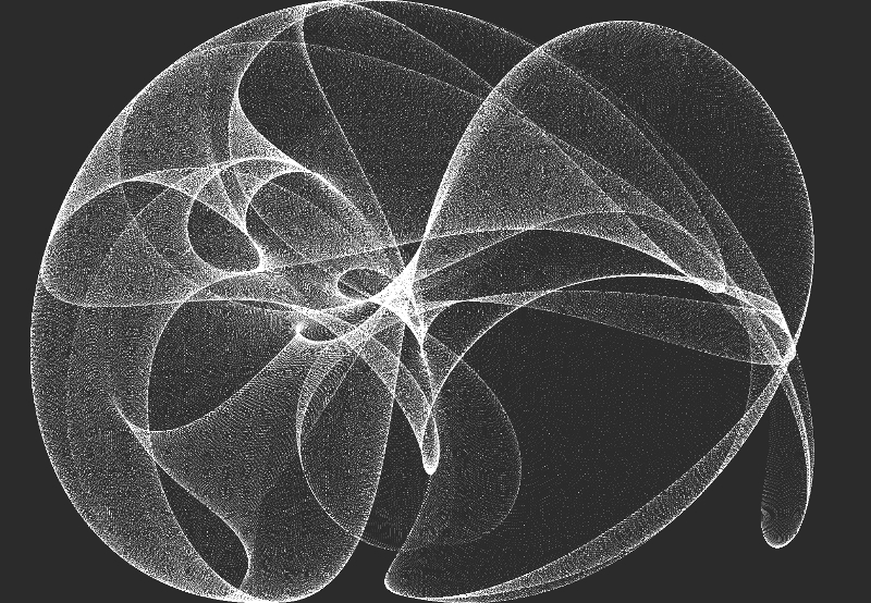 

Postprocessing

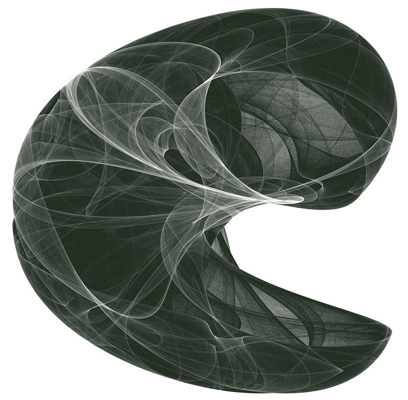
Finally, at the post-processing stage, we will apply several effects.

Gradient mapping . Adds color content based on the brightness of the original image.


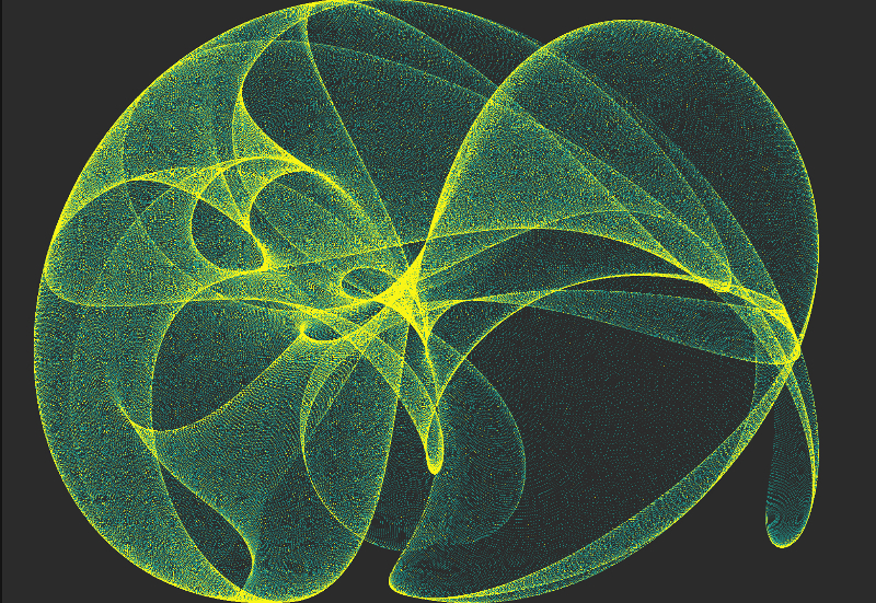
Bloom . Adds a slight glow.

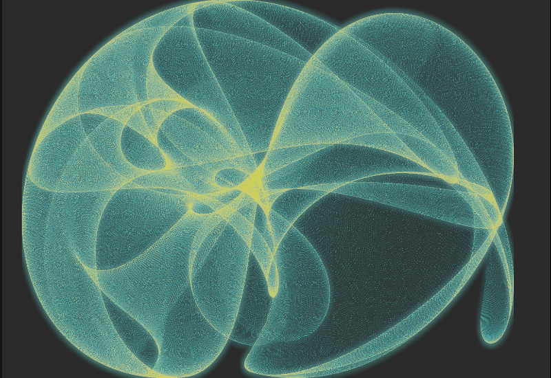
Code

Project repository on GitHub .
Currently available:

• Main code base (C ++ 11 / C ++ 14) along with shaders;
• Examples and demo versions of applications;
  
  • Liquid Fluid simulation;
  • Light Scattered. Adaptation of the effect of scattered light;
  • Strange Attractors. The example described in the article;
  • Wind field. Implementing Navier-Stokes with a large number of particles (2 ^ 20);
  • Flame Simulation. Flame simulation.
• Client for Android.

Continuation

In this example, we see that the computation stage, the stage rendering stage and the post-processing stage consist of several dependent passages.
In the next part, we will try to consider the implementation of multi-pass rendering, taking into account the requirements imposed by each stage.

I would be happy for comments and suggestions (you can mail yegorov.alex@gmail.com)
Thank!