Slowly but surely: choose the optimal strategy for a trading robot

Most of the trading systems created by the type of "cut down money in a hurry." They turn to temporary market inefficiencies in order to make an annual profit of around 100%. For such systems need constant monitoring. They need to be adapted to market conditions. But their lifespan remains relatively short. And, when this time comes, the death of the system is associated, as a rule, with large financial losses. What if you remain a winner but make working with the trading system more comfortable and safe?

We offer you an adapted translation of the article in The Financial Hacker, in which the author rehabilitates Markowitz's idea and his Mean-Variance Optimization approach.
')
The “good old” approach to investing says: buy low-risk assets and wait. Each investment portfolio has a certain average guaranteed income and a certain level of price fluctuations. Usually we seek to minimize the latter and increase the first indicator. The optimal allocation of capital, just, is designed to solve this problem. It implies unequal distribution of invested funds by the number N of assets. The easiest way to solve the problem of increasing average profitability while minimizing risks was suggested 60 years ago by Harry Markowitz . This decision brought him the Nobel Prize.

Outdated Markowitz

Unfortunately, Markowitz was thoroughly forgotten. Although the problem remained: in any trading system, it is necessary to calculate the optimal distribution in retrospect. In real trading, a portfolio optimized in this way mysteriously fails. It is believed that ordinary income in practice is less than 1 / N of capital investments. Recently, an article appeared, the author of which decided to challenge this statement. Here is what the first paragraph of this study says:

“The optimization of the average deviation (MVO), introduced by Markowitz in 1952, is considered today as a beautiful but useless theory in practice. It is called unstable and erroneous procedure. They say that, since it is based on the calculation of average, volatility and correlation of asset returns, then the slightest error at the input makes the use of this optimization meaningless. ”

In fact, putting the correct data at the entrance to the system is not such a big problem. And the calculation parameters themselves are few. But for some reason, such an optimized portfolio among critics Markowitz really does not work. They probably do something wrong. For example, using too long periods of return to the average for the sample. Or they use the MVO algorithm incorrectly, mixing short and long portfolios. With the correct application of periods of momentum and extremely long portfolios of investments, the MVO gives a result outside the sample that is much higher than the 1 / N indicator. Do not believe? See an example of testing this algorithm on R in the blog of Ilya Kipris .

Realization on R is a rare practice in real trading. You should try MVO on another platform. Then you can invest in an optimized stock portfolio or one of the ETFs, allow the platform to balance the distribution of funds at regular intervals, roll back, wait and start earning gradually and thoughtfully.

MVO implementation

To be implemented on Zorro, the author takes the Markowitz layout from a 1959 publication. In Chapter 8, he describes the MVO algorithm in the most comprehensible and accessible way. For not the most advanced programmers, there is even an introduction to linear algebra. The author added to the original algorithm only weight restrictions, as suggested by the authors of the above article. In the end, it turned out that it was a great idea. This condition helped stabilize the algorithm and improved its performance outside the sample.

Anticipating the emergence of fast and smart computers, Markowitz included in the description a set of examples by which you can check whether the algorithm was programmed correctly. This is what this check looks like:

function main() { var Means[3] = { .062,.146,.128 }; var Covariances[3][3] = { .0146,.0187,.0145,.0187,.0854,.0104,.0145,.0104,.0289 }; var Weights[3]; var BestVariance = markowitz(Covariances,Means,3); markowitzReturn(Weights,1); printf("\nMax: %.2f %.2f %.2f",Weights[0],Weights[1],Weights[2]); markowitzReturn(Weights,BestVariance); printf("\nBest: %.2f %.2f %.2f",Weights[0],Weights[1],Weights[2]); markowitzReturn(Weights,0); printf("\nMin: %.2f %.2f %.2f",Weights[0],Weights[1],Weights[2]); }

Here the means and covariances are built into a script taken from a set of examples proposed by Markowitz. The markowitz function starts the algorithm and returns the deviation value associated with the best Sharpe ratio. The markowitzReturn function then calculates the weights (load) of the distribution of capital with the maximum average return for the proposed deviation. The weights for maximum, best and minimum deviations are printed. If we did everything right, these values should coincide with those given in the book Markowitz.

  Max: 0.00 1.00 0.00
 Best: 0.00 0.22 0.78
 Min: 0.99 0.00 0.01

Asset selection

For long-term portfolios, you cannot use high-leverage Forex or CFD tools (leverage) that are suitable for short-term strategies. Instead, you invest in stocks, ETFs, or other similar assets. For algorithmic trading, they have a certain benefit:

A zero-sum game is excluded. In the long run, stocks and ETF indices have a positive return to average value, based on dividends and market trends.
More reliable brokers appear. Brokers working with stocks and ETFs regulate what can not be said about Forex and CFD brokers.
More data to upload to your algorithm. For example, information about the volume and depth of the market.
More asset choices in various market sectors.
More trading methods.

An obvious disadvantage of these tools is low leverage. For example, 1: 4 instead of 1: 100 in the foreign exchange market. Low leverage is suitable for long-term investments, but it cannot be earned quickly. There are a number of other limitations with long-term portfolios. MVO obviously does not work with things that do not have a positive average return. It will not work, even if the income is strongly correlated. Therefore, when choosing assets, it is worth paying attention not only to returns, but also to correlation. Here is an example Zorro script for this task:

 #define NN 30 // max number of assets function run() { BarPeriod = 1440; NumYears = 7; LookBack = NumBars; string Names[NN]; vars Returns[NN]; var Correlations[NN][NN]; int N = 0; while(Names[N] = loop( "TLT","LQD","SPY","GLD","VGLT","AOK")) { if(is(INITRUN)) assetHistory(Names[N],FROM_YAHOO); asset(Names[N]); Returns[N] = series((priceClose(0)-priceClose(1))/priceClose(1)); if(N++ >= NN) break; } if(is(EXITRUN)) { int i,j; for(i=0; i<N; i++) for(j=0; j<N; j++) Correlations[N*i+j] = Correlation(Returns[i],Returns[j],LookBack); plotHeatmap("Correlation",Correlations,N,N); for(i=0; i<N; i++) printf("\n%i - %s: Mean %.2f%% Variance %.2f%%", i+1,Names[i], 100*annual(Moment(Returns[i],LookBack,1)), 252*100*Moment(Returns[i],LookBack,2)); } }

To begin with, he sets a number of parameters, then starts a cycle with N assets. Here, for example, are the most popular ETF. There is a website etfdb.com , which will help you to replace them with the optimal combination.

At the first launch, asset prices were downloaded from Yahoo. The assetHistory function saves them as historical data. Then assets are selected, their returns are counted, and this data is already stored in the Returns data series. This procedure is repeated on every day of the 7 years of the test period (in practice, it all depends on when the selected ETF assets become available). As a result, the script prints the annual values of the average return and deviations of each asset. They become, respectively, the first and second moment each series. The annual function and the multiplier 252 convert daily values to annual values. In our example, the result is the following:

  1 - TLT: Mean 10.75% Variance 2.29%
 2 - LQD: Mean 6.46% Variance 0.31%
 3 - SPY: Mean 13.51% Variance 2.51%
 4 - GLD: Mean 3.25% Variance 3.04%
 5 - VGLT: Mean 9.83% Variance 1.65%
 6 - AOK: Mean 4.70% Variance 0.23%

An ideal ETF will have a high return on average, a low deviation and a weak correlation with other assets in the sample. The correlation can be seen in the correlation matrix, which is calculated for all collected return values and is drawn in the form of a thermal diagram N * N.

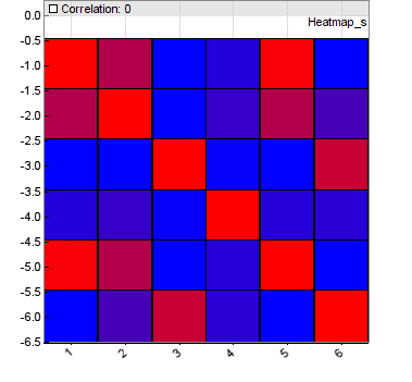
The matrix contains the correlation coefficient of each asset in relation to each other asset. In our case, there are 6 of them. Blue is for weak correlation, red is therefore high. From this diagram it is clear that some assets should not have been chosen.

Efficiency limit

After choosing the assets in our portfolio, it's time to calculate the optimal distribution of capital in it through the MVO algorithm. In any case, “optimality” depends on the assumption of risks. In other words, portfolio volatility. For each of the risk values, there is an optimal distribution, which generates the maximum profit. That is, the optimal distribution is not a frozen point, but rather a curve in the return / deviation graph. It is also called the limit or the limit of efficiency. We can calculate it and draw it in the form of a diagram using the following script:

  function run() { ... // similar to Heatmap script if(is(EXITRUN)) { int i,j; for(i=0; i<N; i++) { Means[i] = Moment(Returns[i],LookBack,1); for(j=0; j<N; j++) Covariances[N*i+j] = Covariance(Returns[i],Returns[j],LookBack); } var BestV = markowitz(Covariances,Means,N); var MinV = markowitzVariance(0,0); var MaxV = markowitzVariance(0,1); int Steps = 50; for(i=0; i<Steps; i++) { var V = MinV + i*(MaxV-MinV)/Steps; var R = markowitzReturn(0,V); plotBar("Frontier",i,V,100*R,LINE|LBL2,BLACK); } plotGraph("Max Sharpe",(BestV-MinV)*Steps/(MaxV-MinV), 100*markowitzReturn(0,BestV),SQUARE,GREEN); } }

Let's skip the first part of it, it is identical to the code for creating a heat map. Only in this case the covariance matrix is calculated. The covariances and returns of the average are entered into the markowitz function, which again makes the deviation return, based on the best Sharpe ratio. That in turn refers to the markowitzVariance , there is a return of the higher and lower deviations of the limit of efficiency. Get the boundaries of the graph. As a result, the script produces 50 points of annual return of the average from the lowest to the highest deviations: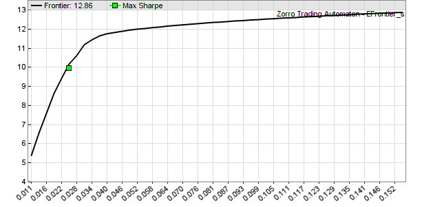

On the right, we can see how the portfolio reaches its maximum annual profit rate of 12.9%. On the left, we have a value of 5.4%, but with the number of daily deviations less than 10. The green dot on the graph indicates the best Sharpe ratio (profit divided by the square root of deviations) from 10% of annual income with a deviation of 0.025. This is the optimal portfolio. At least in retrospect data.

Experiment

How does our optimized average / deviation portfolio behave within the sample and beyond the sample in comparison with 1 / N? Below is a script for experimental verification with differently assembled portfolios, rollback periods, weight restrictions and deviations:

 #define DAYS 252 // 1 year lookback period #define NN 30 // max number of assets function run() { ... // similar to Heatmap script int i,j; static var BestVariance = 0; if(tdm() == 1 && !is(LOOKBACK)) { for(i=0; i<N; i++) { Means[i] = Moment(Returns[i],LookBack,1); for(j=0; j<N; j++) Covariances[N*i+j] = Covariance(Returns[i],Returns[j],LookBack); } BestVariance = markowitz(Covariances,Means,N,0.5); } var Weights[NN]; static var Return, ReturnN, ReturnMax, ReturnBest, ReturnMin; if(is(LOOKBACK)) { Month = 0; ReturnN = ReturnMax = ReturnBest = ReturnMin = 0; } if(BestVariance > 0) { for(Return=0,i=0; i<N; i++) Return += (Returns[i])[0]/N; // 1/N ReturnN = (ReturnN+1)*(Return+1)-1; markowitzReturn(Weights,0); // min variance for(Return=0,i=0; i<N; i++) Return += Weights[i]*(Returns[i])[0]; ReturnMin = (ReturnMin+1)*(Return+1)-1; markowitzReturn(Weights,1); // max return for(Return=0,i=0; i<N; i++) Return += Weights[i]*(Returns[i])[0]; ReturnMax = (ReturnMax+1)*(Return+1)-1; markowitzReturn(Weights,BestVariance); // max Sharpe for(Return=0,i=0; i<N; i++) Return += Weights[i]*(Returns[i])[0]; ReturnBest = (ReturnBest+1)*(Return+1)-1; plot("1/N",100*ReturnN,AXIS2,BLACK); plot("Max Sharpe",100*ReturnBest,AXIS2,GREEN); plot("Max Return",100*ReturnMax,AXIS2,RED); plot("Min Variance",100*ReturnMin,AXIS2,BLUE); } }

The verification cycle is 7 years of historical data. It stores daily returns in a series of Returns data. On the first trading day of each month (tdm() == 1) matrices of averages and covariances for the last 252 days are calculated. On their basis, the limit of efficiency is measured. In our case, the weight limit is 0.5 relative to the minimum deviation point. If we take this efficiency limit as a basis, we get a daily total profit with the same weight ( ReturnN ), the best Sharpe ratio ( ReturnBest ), the minimum deviation ( ReturnMin ) and the maximum income ( ReturnMax ). The weight remains unchanged until the next balancing, when we pass the test outside the sample. Profits for 4 days are added to 4 different stock curves: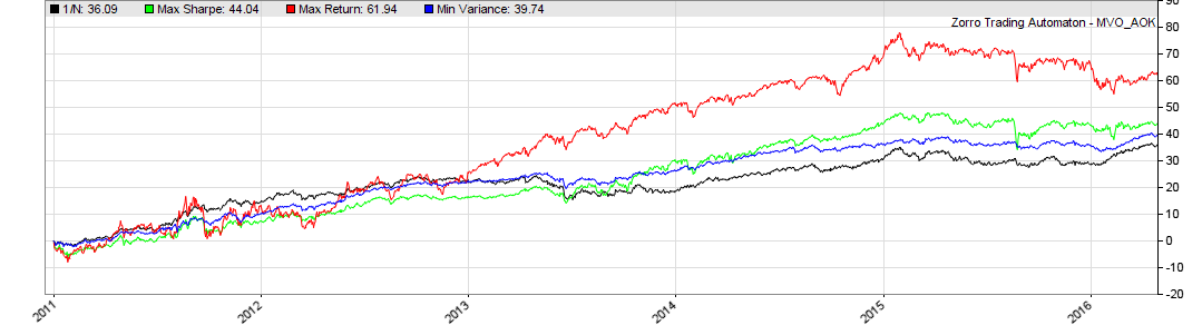

From the chart you can see that the MVO has improved the portfolio for all three options, despite its poor reputation. The black line marks 1 / N portfolio with the same weight for each asset. The blue line indicates a portfolio with a minimum deviation. We see that its return is higher than 1 / N, with much lower volatility. The red line is a portfolio with maximum yield but high volatility. The green line is the best Sharpe ratio, it is an average portfolio for all indicators. The composition of the portfolio may be different, but the green and blue lines show the best options.

To check the monthly balancing of the distribution of scales, you can display them in the form of a heat map.

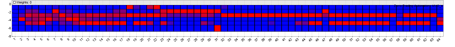
The horizontal axis denotes the monthly period of our simulation. Vertical - asset number. High weights are painted in red, lower weights are in blue. This is the distribution of weights for a portfolio with a maximum Sharpe ratio consisting of 6 ETF assets.

"We bring" in system money

After all the experiments, you can encode a long-term system. The following procedure is proposed for this:

The efficiency limit is calculated based on the daily profit of the last 252 trading days. That is one year. This is the best period, according to the article we quoted at the beginning. Since most ETFs demonstrate annual momentum.
The portfolio is balanced once a month. In tests, shorter periods have shown their worthlessness, and they have reduced revenue due to higher trading costs. With longer periods (3 months), the system performance deteriorates.
The point of the limit of efficiency can be made floating within the limits of the minimum deviation and maximum Sharpe ratio. So you can control the risk level of the system.
We use a 50% weight limit for minimum deviation. This is not the most optimal portfolio, but, again, in the cited article (and the author’s tests have confirmed this), it is said that this improves the balance outside the sample.

Here is the script:

 #define LEVERAGE 4 // 1:4 leverage #define DAYS 252 // 1 year #define NN 30 // max number of assets function run() { BarPeriod = 1440; LookBack = DAYS; string Names[NN]; vars Returns[NN]; var Means[NN]; var Covariances[NN][NN]; var Weights[NN]; var TotalCapital = slider(1,1000,0,10000,"Capital","Total capital to distribute"); var VFactor = slider(2,10,0,100,"Risk","Variance factor"); int N = 0; while(Names[N] = loop( "TLT","LQD","SPY","GLD","VGLT","AOK")) { if(is(INITRUN)) assetHistory(Names[N],FROM_YAHOO); asset(Names[N]); Returns[N] = series((priceClose(0)-priceClose(1))/priceClose(1)); if(N++ >= NN) break; } if(is(EXITRUN)) { int i,j; for(i=0; i<N; i++) { Means[i] = Moment(Returns[i],LookBack,1); for(j=0; j<N; j++) Covariances[N*i+j] = Covariance(Returns[i],Returns[j],LookBack); } var BestVariance = markowitz(Covariances,Means,N,0.5); var MinVariance = markowitzReturn(0,0); markowitzReturn(Weights,MinVariance+VFactor/100.*(BestVariance-MinVariance)); for(i=0; i<N; i++) { asset(Names[i]); MarginCost = priceClose()/LEVERAGE; int Position = TotalCapital*Weights[i]/MarginCost; printf("\n%s: %d Contracts at %.0f$",Names[i],Position,priceClose()); } } }

The script itself only “advises”, but does not trade. To automate the process, you still need to integrate the trading robot through the brokerage system API (for example, ITinvest called this interface SmartCOM ). At the same time, if positions are opened and closed once a month, and data on promotions can be found in open access, then integration may not be necessary - you just need to run it once a month and analyze its output:

  TLT: 0 Contracts at $ 129
 LQD: 0 Contracts at $ 120
 SPY: 3 Contracts at $ 206
 GLD: 16 Contracts at $ 124
 VGLT: 15 Contracts at $ 80
 AOK: 0 Contracts at $ 32

Obviously, the optimal portfolio for this month will consist of three deals on SPY, 16 on GLD and 15 VGLT. Now you can manually open and close positions in your brokerage platform until the portfolio matches the printed list. Leverage by default - 4. But it can be changed at will at the beginning of the script (# define). If you want to make the script trade independently, replace the printf command with a command to open and close positions.

MVO vs OptimalF

MVO can be used not only for a portfolio with a certain number of assets, but also for different trading systems. The author of the Financial blog conducted an experiment, during which it turned out that MVO does not exceed the result that can be obtained by applying the OptimalF coefficient of Ralph Vins. It is used in most trading systems. OptimalF does not perform correlations between components, but takes into account the depth of sampling of funds. While MVO works only with averages and covariances. The ideal solution would be to combine both approaches - but this is a matter for future experiments.