As a programmer, I bought a car
Recently, I was puzzled by the search B. car, in exchange for just sold, and, as is usually the case, several competitors claimed this role.
As you know, for the purchase of cars on the territory of the Russian Federation there are several large reputable sites (auto.ru, drom.ru, avito.ru), on which I gave preference. My requirements were met by hundreds, and for some models, thousands of cars from the sites listed above. Apart from the fact that it is inconvenient to search on several resources, I would also like to select the most profitable (the price of which relative to the market is undervalued) proposals for a priori information that each resource provides before going to watch the car “live”. Of course, I really wanted to solve several overdetermined systems of algebraic equations (possibly nonlinear) of high dimension manually, but I overpowered myself and decided to automate this process.

I collected data from all the resources described above, and I was interested in the following parameters:
I noted the data not filled by lazy sellers as NA (Not Available) so that these values could be correctly processed with R.
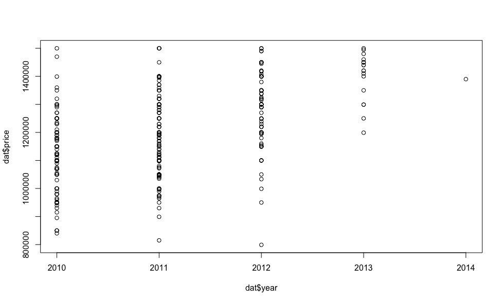
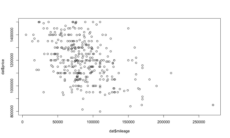
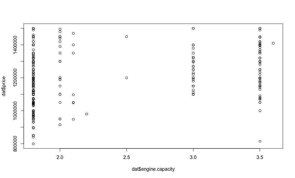
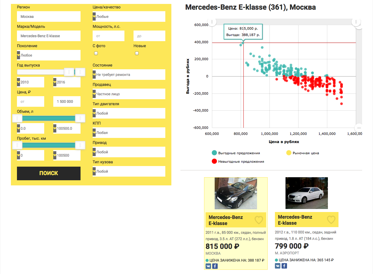
In order not to go into the dry theory, let's look at a specific example, we will look for profitable Mercedes-Benz E-klasse not older than the 2010 release, worth up to 1.5 million rubles in Moscow. In order to start working with data, first of all we fill in the missing values (NA) for medians, the benefit for which in R is the median () function.
, .
( ).
2013 2014!
, , .

— , , .
, , , “”, , .
, , .
, , , , .
, -:
, , , . , , .
, - , , , .
?
, 59% , , «», .. , . 4- ( 28%) , .
, , , , , (, , , , , , ), . , , , .
, , 3 :
:
1. csv — dataset.txt
As you know, for the purchase of cars on the territory of the Russian Federation there are several large reputable sites (auto.ru, drom.ru, avito.ru), on which I gave preference. My requirements were met by hundreds, and for some models, thousands of cars from the sites listed above. Apart from the fact that it is inconvenient to search on several resources, I would also like to select the most profitable (the price of which relative to the market is undervalued) proposals for a priori information that each resource provides before going to watch the car “live”. Of course, I really wanted to solve several overdetermined systems of algebraic equations (possibly nonlinear) of high dimension manually, but I overpowered myself and decided to automate this process.
Data collection
I collected data from all the resources described above, and I was interested in the following parameters:
- price (price)
- year of manufacture
- mileage
- engine capacity (engine.capacity)
- engine power (engine.power)
- engine type (2 indicator mutually exclusive variables diesel and hybrid, taking the values 0 or 1, for diesel and hybrid engines, respectively). The default engine type is gasoline (not rendered into the third variable in order to avoid multicollinearity ).
')
In this way: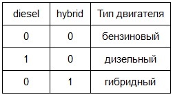
Further, similar logic for indicator variables is implied by default. - type of gearbox (indicator variable mt (manual transmission), which takes a boolean value, for a manual transmission). The type of gearbox is automatic by default.
It should be noted that I referred to automatic transmissions as not only a classic hydraulic automatic, but also robotic mechanics and a CVT. - drive type (2 indicator variables front.drive and rear.drive, taking boolean values). The default drive type is full.
- body type (7 indicator variables sedan, hatchback, wagon, coupe, cabriolet, minivan, pickup, taking boolean values). Body type default - SUV / crossover
I noted the data not filled by lazy sellers as NA (Not Available) so that these values could be correctly processed with R.
Data visualization
In order not to go into the dry theory, let's look at a specific example, we will look for profitable Mercedes-Benz E-klasse not older than the 2010 release, worth up to 1.5 million rubles in Moscow. In order to start working with data, first of all we fill in the missing values (NA) for medians, the benefit for which in R is the median () function.
dat <- read.csv("dataset.txt") #    R

dat$mileage[is.na(dat$mileage)] <- median(na.omit(dat$mileage)) #
, .
( ).
2013 2014!
, , .
— , , .
, , , “”, , .
, , .
, , , , .
, -:
- , ..:
- .(. ), .
- ., :
dat_cor <- as.matrix(cor(dat)) #

dat_cor[is.na(dat_cor)] <- 0 #     0 (..          )

library(corrplot) #   corrplot,

palette <-colorRampPalette(c("#7F0000","red","#FF7F00","yellow","#7FFF7F", "cyan", "#007FFF", "blue","#00007F"))

corrplot(dat_cor, method="color", col=palette(20), cl.length=21,order = "AOE", addCoef.col="green") #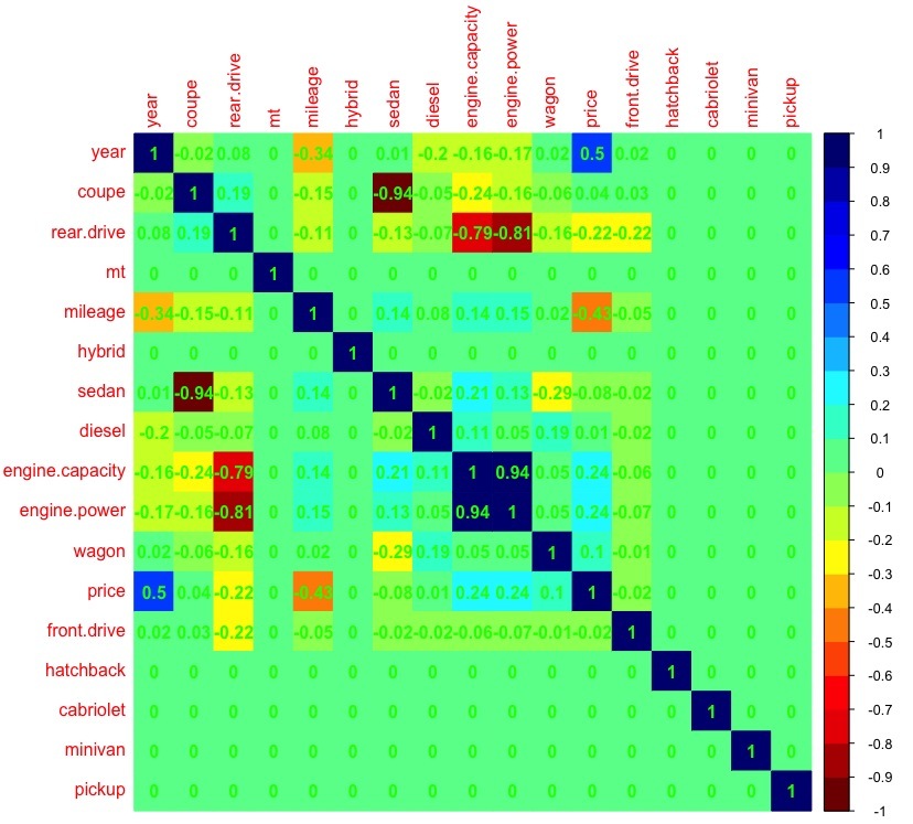
(>0.7) , engine.capacity, .. ( , , — ). - .— (. ), . , , — , , , .
. , , dffits, (covratio), , i- , . , dfbetas, i- .
(covratio) — . i- .
, , , dffits.
— , .. , .
, dffits covratio.model <- lm(price ~ year + mileage + diesel + hybrid + mt + front.drive + rear.drive + engine.power + sedan + hatchback + wagon + coupe + cabriolet + minivan + pickup, data = dat) # model.dffits <- dffits(model) # dffits
dffits 2*sqrt(k/n) = 0.42, (k — , n — ).model.dffits.we <- model.dffits[model.dffits < 0.42] model.covratio <- covratio(model) #
covratio | model.covratio[i] -1 | > (3*k)/n.model.covratio.we <- model.covratio[abs(model.covratio -1) < 0.13] dat.we <- dat[intersect(c(rownames(as.matrix(model.dffits.we))), c(rownames(as.matrix(model.covratio.we)))),] # model.we <- lm(price ~ year + mileage + diesel + hybrid + mt + front.drive + rear.drive + engine.power + sedan + hatchback + wagon + coupe + cabriolet + minivan + pickup, data = dat.we) #
, , .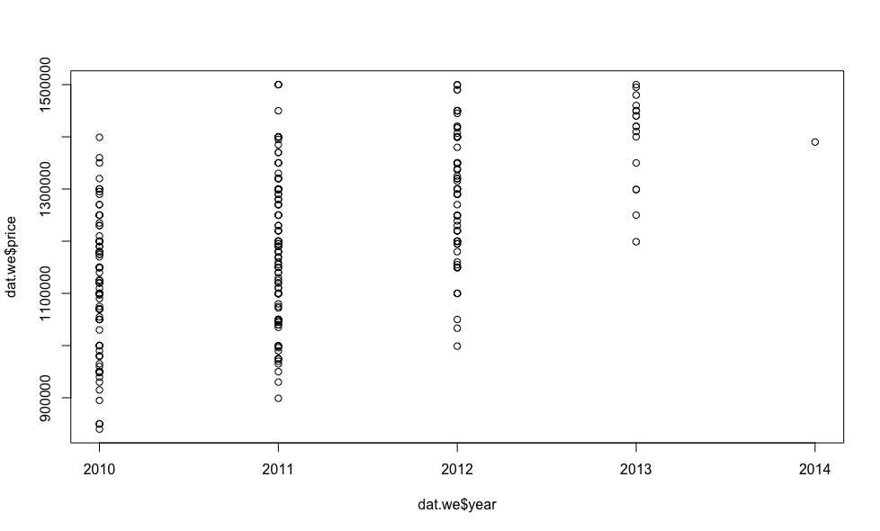

, 18 , .
- .
- ..
- , ()( R resid()).
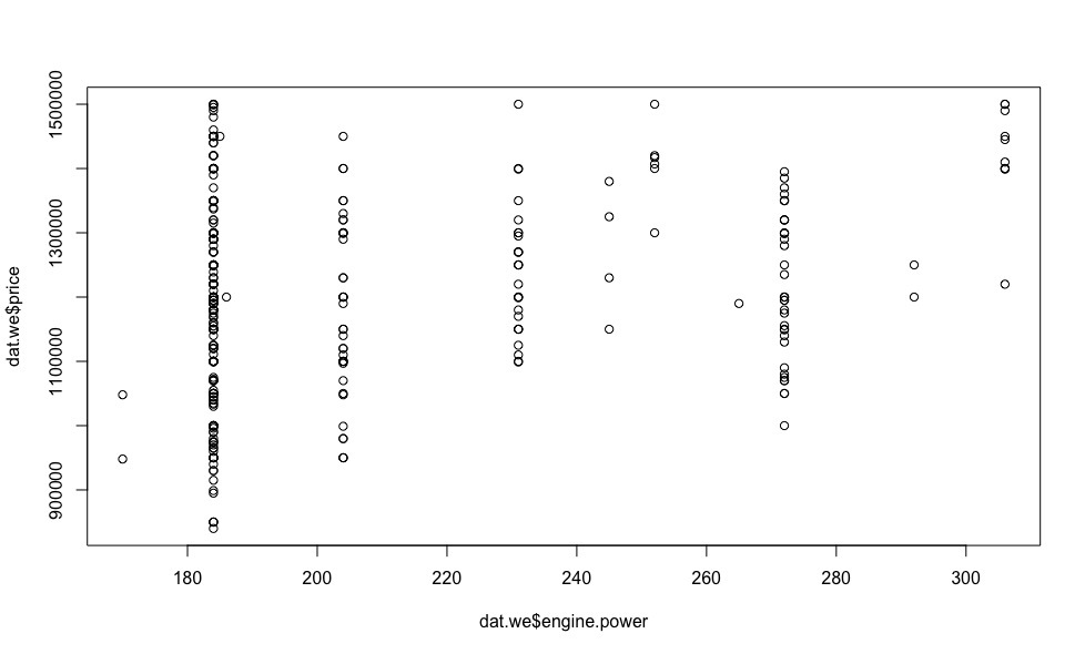
plot(dat.we$year, resid(model.we))
plot(dat.we$mileage, resid(model.we))
plot(dat.we$engine.power, resid(model.we))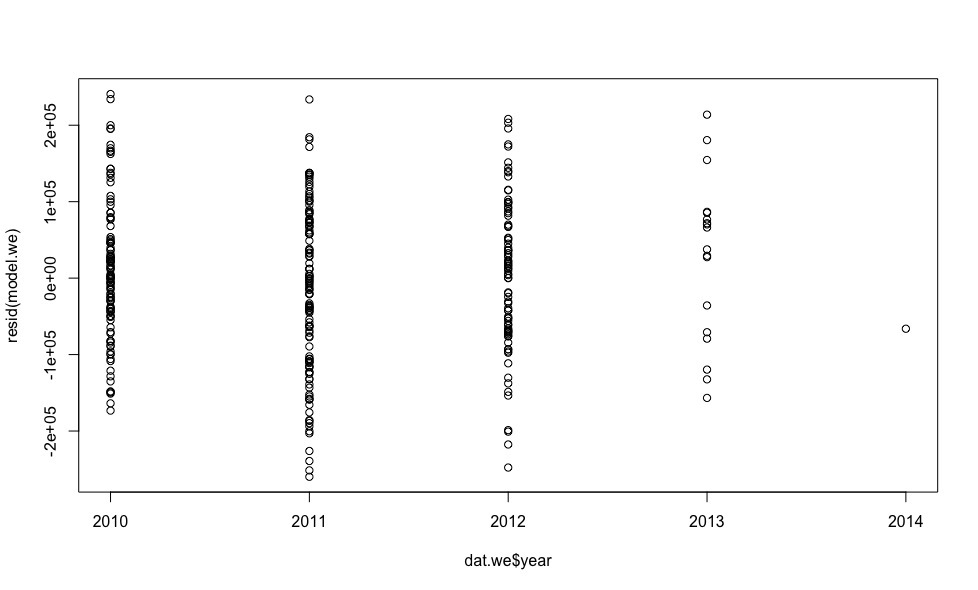
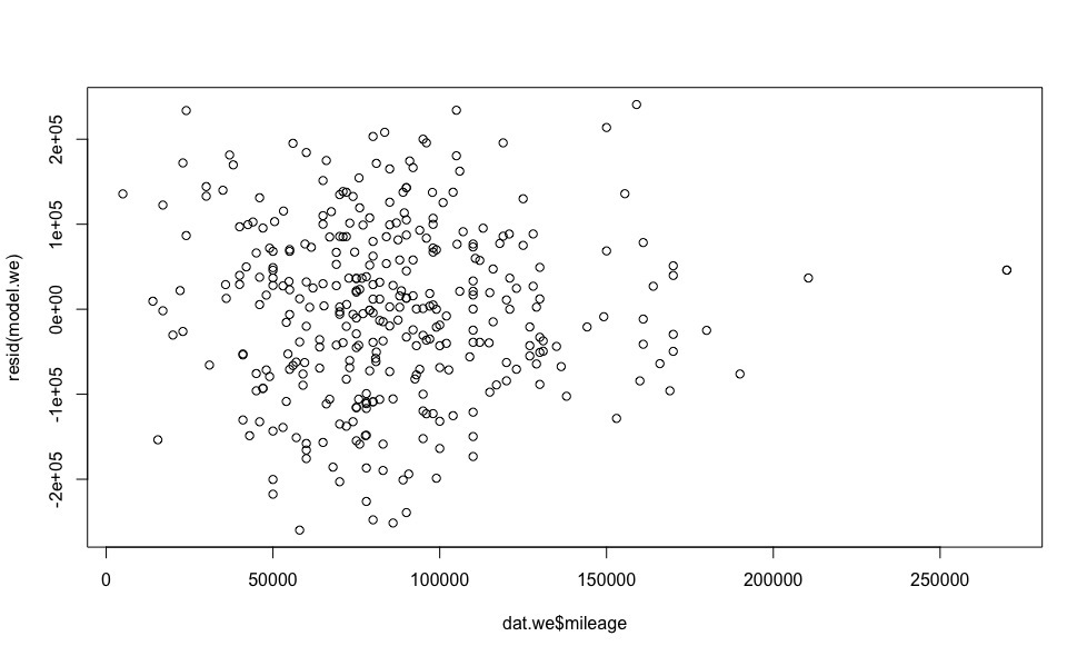
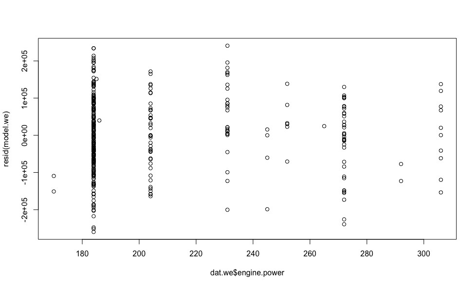
- , . - ., , .
qqnorm(resid(model.we))
qqline(resid(model.we))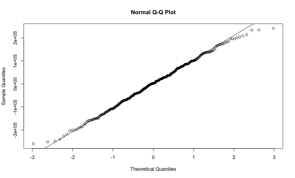
, , , . , , .
model.we <- lm(price ~ year + mileage + diesel + hybrid + mt + front.drive + rear.drive + engine.power + sedan + hatchback + wagon + coupe + cabriolet + minivan + pickup, data = dat.we)
coef(model.we) #
(Intercept) year mileage diesel rear.drive engine.power sedan
-1.76e+08 8.79e+04 -1.4e+00 2.5e+04 4.14e+04 2.11e+03 -2.866407e+04
predicted.price <- predict(model.we, dat) #
real.price <- dat$price #
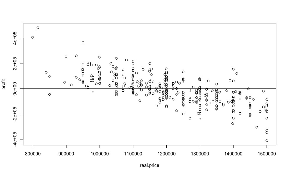
profit <- predicted.price - real.price #
, - , , , .
plot(real.price,profit)
abline(0,0)
?
sorted <- sort(predicted.price /real.price, decreasing = TRUE)
sorted[1:10]
      69       42      122      248      168       15      244      271      109      219
1.590489 1.507614 1.386353 1.279716 1.279380 1.248001 1.227829 1.209341 1.209232 1.204062
, 59% , , «», .. , . 4- ( 28%) , .
, , , , , (, , , , , , ), . , , , .
, , 3 :
- ?
- ?
- ?
:
- 80/20.
set.seed(1) #     ( )

split <- runif(dim(dat)[1]) > 0.2 #

train <- dat[split,] #

test <- dat[!split,] #

train.model <- lm(price ~ year + mileage  + diesel + hybrid + mt + front.drive + rear.drive + engine.power + sedan + hatchback + wagon + coupe + cabriolet + minivan + pickup, data = train) #

train.dffits <- dffits(train.model) #   dffits

train.dffits.we <- train.dffits[train.dffits < 0.42] #     dffits

train.covratio <- covratio(train.model)  #

train.covratio.we <- model.covratio[abs(model.covratio -1) < 0.13] #     covratio

train.we <- dat[intersect(c(rownames(as.matrix(train.dffits.we))), c(rownames(as.matrix(train.covratio.we)))),] #

train.model.we <- lm(price ~ year + mileage  + diesel + hybrid + mt + front.drive + rear.drive + engine.power + sedan + hatchback + wagon + coupe + cabriolet + minivan + pickup, data = train.we) #

predictions <- predict(train.model.we, test) #

print(sqrt(sum((as.vector(predictions - test$price))^2)/length(predictions))) #     ( )
[1] 121231.5
— . - , , .
2 ( ) .
. - , -, .
, — Mercedes-Benz E-klasse 2010 , 1.5 . .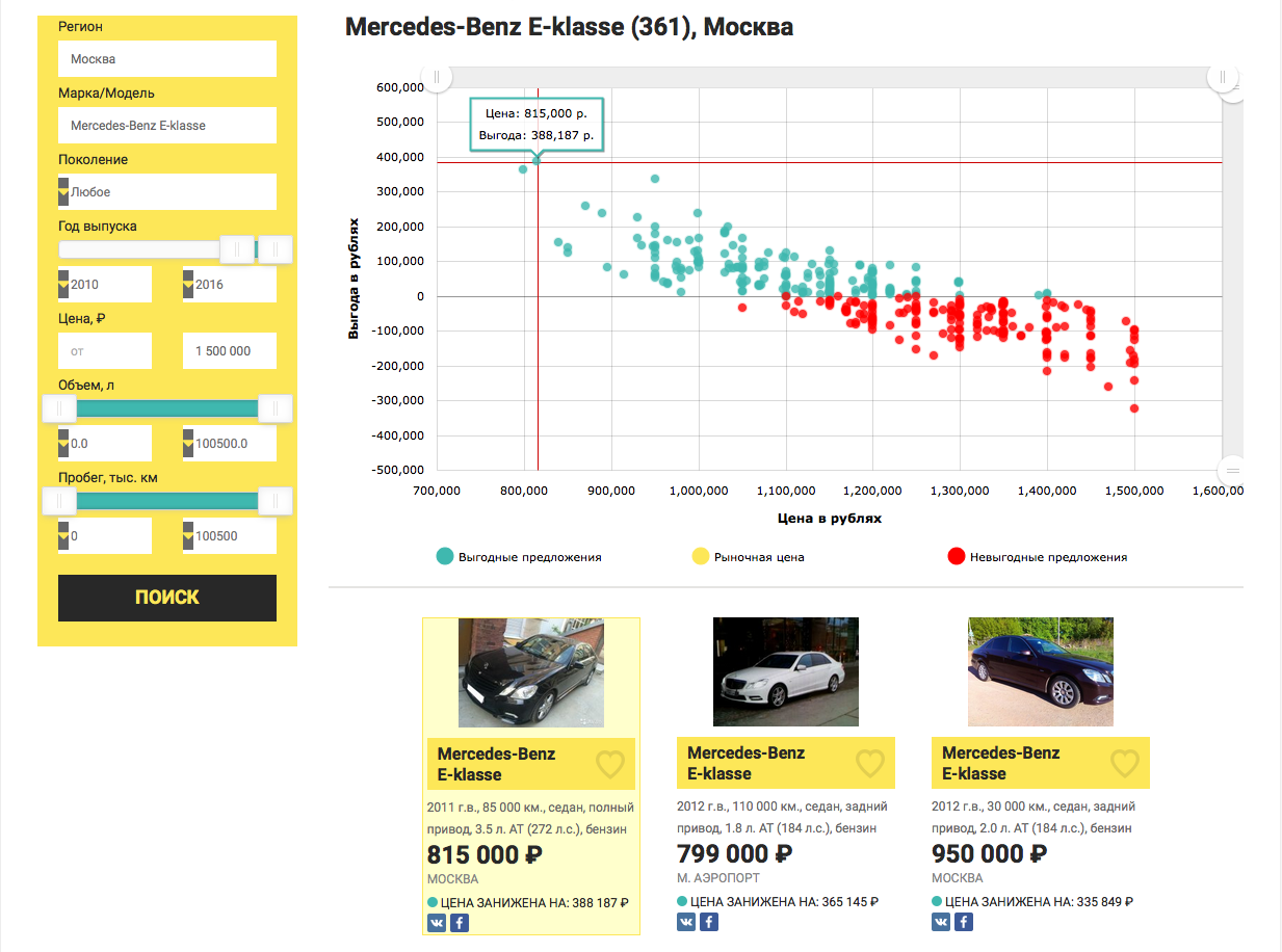
1. csv — dataset.txt
Source: https://habr.com/ru/post/302788/
All Articles