Object data recognition system
DISPLAY SYSTEM OF DISPLAYED DATA OF OBJECT
INTRODUCTION
The developed system is designed for contactless recognition of object data displayed on its display. The system is part of the means to test the object according to the dialogue between the object and the user.
Testing systems with access to software or hardware channels for displaying user information does not require data recognition. However, when such a connection to the object data is missing, it can be performed using a contactless recognition system, which can provide long-term monitoring of the state of the object in automatic mode.
This paper discusses the MatLAB recognition tools without using neural networks, the effectiveness of which, to a large extent, depends on the learning outcomes.
The features of the developed system are shown on the example of data recognition of the diving computer of Open Safety Equipment Ltd.
The article contains the following sections.
• MatLAB image processing library functions
• Characteristics of the used web camera, connecting the camera to the MatLAB environment, setting up camera modes.
• Character recognition using correlation functions.
• Recognition User Interface and Recognition Results
LIBRARY FUNCTIONS OF IMAGE PROCESSING OF MATLAB
MatLAB has libraries of functions for working with graphic files and video signals. Below are given the options used library functions.
Reading image image file

Fig. 1. RGB image [1] jpg file format <196x259x3 uint8>
Supported input file formats are BMP, CUR, GIF, HDF4, ICO, LPEG, JPEG 2000, PBM, PCX, PGM.
')
Adding a graphic primitive to an image
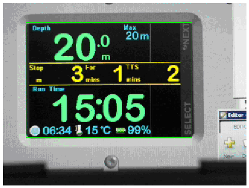
Fig. 2. The pct image with a rectangular green frame, <240x320x3 uint8>.
The m-code for adding primitives to video frames:

Fig. 3. Video image with added geometric primitives.
Image reduction
Image reduction 2N times is achieved by a corresponding decrease in the number of image pixels for each coordinate.

Fig. 4. Image reduction 4 times.
Image resizing
Selection of a fragment of the image
Convert RGB Image to Gray Palette

Fig. 5. Reduction of RGB images to grayscale.
Image filtering
2d median image filtering in grayscale
Blur image
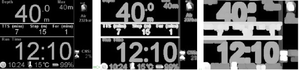
Fig. 6. Examples of blur left image.
Thinning of the solid elements of the image
Fig. 7. An example of thinning solid image elements.
Subtracting a constant from an image or another image
Image preparation and subtraction program:

Fig. 8. Result (on the right) of subtracting the average image from the left.
Convert matrix to gray tones
2d bundle

Fig. 9. The action of convolution.
Image intensity scaling

Fig. 10. Scaling intensity.
Conversion of a numeric matrix into a logical
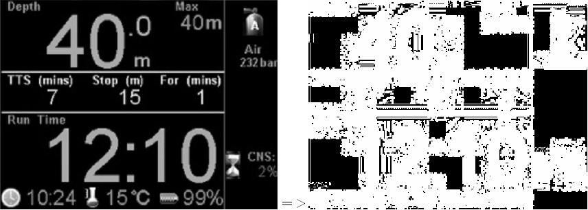
Fig. 11. Convert <196 x 256 double> matrices to binary <196 x 256 logical>
Fill contoured elements

Fig. 12. Fill elements with continuous contours <196 x 256 double>
Removal of solid (island) fragments (noise) from a binary image

Fig. 13. Removal of “black == 0” fragments larger than 500 pixels using the NOT inversion.
Program Code:
Selection of fragments (islands) of the binary image

Fig. 14. Fragment of ten numbered “island” groups of units of the binary image.
Finding the coordinates and sizes of island zones

Fig. 15. A fragment of a graphical representation of the Iprops structural variable containing the coordinates and dimensions of rectangular zones of numbered groups and the binary matrix of each group. Selected coordinates and sizes of the fifth group.
bar chart
The imhist histogram (Img_reference) allows you to get the dependence of the number of pixels for each intensity.

Fig. 16. Image (left) and its histogram - the number of gray tones. The histogram shows that black color of zero intensity prevails in the image: ~ 3500 points.
Intensity distribution

Fig. 17. The total intensity distribution in rows sum (Img).
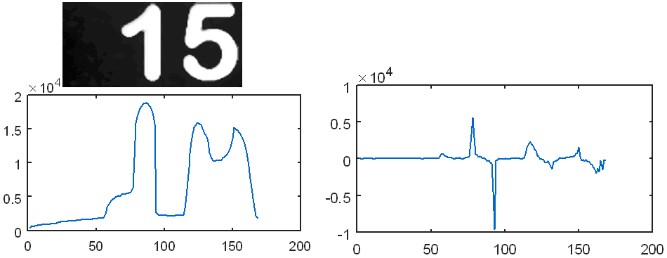
Fig. 18. On the left - the sum of the intensity of pixels in the rows sum (Img) after the median filter Img = medfilt2 (Img, [5 5]). On the right is the derivative of the sum diff (sum (Img)).
Three-dimensional construction of video images.
Video frame can be presented in tabular form, as shown in Fig. 19 for character 9.

Fig. 19. Tabular distribution of the pixel intensity of the character "9" in Excel.
Plotter MatLAB has a “Rotate 3D” button (Fig. 20), which allows displaying output data in 3d format.

Fig. 20. Button plotter to convert the displayed data in 3d format.
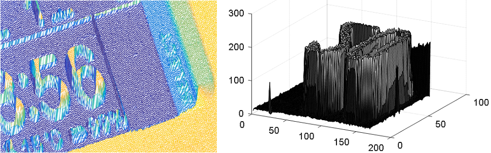
Fig. 21. Examples of 3d images. The right shows the characters "20". Vertical displays pixel intensity.
VIDEO CAMERA
The project used a high-definition webcam HD Logitech C52 [2].
Specifications camcorder Logitech C52.
• HD video communication (1280 x 720 pixels)
• HD video: up to 1280 x 720 pixels.
• Autofocus
• Photos: up to 8 megapixels (with software processing)
• Built-in microphone with Logitech RightSound technology

Fig. 22. Appearance and settings of the camcorder Logitech C52.
Basic computer requirements with a camera resolution of 1280 x 720 pixels.
• 2.4 GHz processor frequency
• RAM capacity 2 GB
• 200 MB free hard disk space
• USB 2.0 port
• Operating environment: Windows XP (SP2 or higher), Vista or Windows 7 (32-bit or 64-bit)
Connect camcorder to Matlab
1. Check if the camcorder is on the MatLAB device list.
2. If the camera is not listed, connect it using the Support Package Installer package (see Fig. 23)

Fig. 23. Connecting the camcorder to MATLAB.
3. After successful installation, the camera is listed
Connect camcorder to Simulink
National Instruments camcorders can connect to the SimLink MatLAB environment via the Image Acquisition Toolbox> From Video Device library objects. To connect, you must install the NI-DAQmx package using the Support Package Installer (Figure 23).
You can run the Image Acquisition Tool from the MatLAB command line:
The procedure for entering video in MatLAB
Input frames in MatLAB performed in the following order.
1. Search for video cameras recognized by MATLAB connected to a computer.
2. Creating a camera object.
3. View RGB video with the output of the camera name, video time, resolution and frame rate.

Fig. 24. Video output in MATLAB.
4. Set the required camera settings.
Examples of the structural list of camera parameters:
Obtain possible parameter values, such as camera resolution

Fig. 25. Images at a resolution of '320x240' '640x480' and '1280x960' pixels.
Setting the required parameter value
5. Exit video viewing mode.
>> closePreview (cam)
6. Frame input.
7. Frame display.
8. Delete the camera object.
Adjusting the position of the camera relative to the object
A frame with known coordinates is added to the video output in the MatLAB (Fig. 26). When adjusting the camera position relative to the object, the object borders should coincide with the frame position.

Fig. 26. The frame in the video frame.
An example of an m-code for displaying a video with a base frame:
Features of the state of the object
During operation, the device changes the format of the information displayed on the screen. The system recognizes a format change by the presence / absence of the TTS and Step fields. For the field of each format, their own distribution of character definition zones has been built. 27.

Fig. 27. Different formats of information displayed by the device under test.
TEXT RECOGNISING
OCR function Matlab
The Optical Character Recognition (OCR) function MatLAB recognizes the text of a graphic file.

Fig. 28. Symbol search zones (23 rectangular zones are highlighted in red), coordinates and dimensions of the zones in results.WordBoundingBoxes.
Table 1. The text recognition result.

An example of automatic detection of text zones and text recognition in MatLAB
An example of automatic text recognition in the MatLAB is shown in the Help section of the Matlab [3].

Fig. 29. Original image [3].
Finding a fragment of the image by the correlation function
The calculation of the normalized cross-correlation norm_Corr_f allows you to track the presence of specified fragments and their coordinates in frames of the video image. This can be used, for example, when searching or counting objects or setting the camera position.
Examples of the implementation of the detection algorithm are shown in Fig. 30, Fig. 31, algorithm code [4].

Fig. 30. Object area - text “Run Time”, correctly detected on the left frame. When you cover the object area with your hand, the search program found the wrong area of the object (right frame).

Fig. 31. The dependence of the correlation function of the frame number. The value of the function in the presence of the object to be searched is ~ 0.99, and in the absence of it, ~ 0.978. The small range of the 0.012 function change makes the search algorithm sensitive to the effects of interference — finding non-object zones that are well correlated with the reference object ...
Improving the signal-to-noise correlation ratio by increasing the ratio of the character area to the character detection area
The ability to distinguish characters by the correlation method depends on the resolution of the character field, the ratio of the character area to the character detection area, and the difference between the designated and reference characters. The correlation increases with increasing resolution and area ratios and decreasing differences between the compared characters.

Fig. 32. The selection of the location of characters.

Fig. 33. The correlation coefficient between the figures of the object 5 (blue line), 6 (brown line) and 2 (yellow line) in the area of 17x25 pixels and reference symbols: empty zone, characters from 0 to 9. The correlation amplitude shows that the pair of two is well different from the rest of the characters (it is easier to detect), and the five differs little from the six.

Fig. 34. The correlation coefficients between the two empty zones of the object and the zone with 9 and the reference symbols "empty"; 0; one; 2; 3; four; five; 6; 7; eight; 9. The graphs show the maximum correlation with the “empty” reference symbol for the first two positions and with the reference 9 for the last position.
Eliminate uncertainty when comparing a symbol with an empty zone
The correlation function can give an undefined value NaN when comparing an object symbol with an empty reference zone consisting of zeros. To eliminate this effect, the intensity of one element of the standard is increased to 255:
Increase correlation using generic fonts
In this version of 320 x 240 pixels, the fonts of the following sizes are 18; 26; 36 and 60. It is possible to select and modify the font of the standard to the object's font using special programs, for example, GLCDFontCreator.exe [5].

Fig. 35. Original image (left) and the result of the imposition of 'Arial Rounded MT Bold' fonts on the original image (right).

Fig. 36. Option narrowing of the search zones of characters.

Fig. 37. Options for reference numbers of high and low resolution. The correlation (coincidence) between the numbers 5 and 6 is higher than between the other characters.

Fig. 38. Pixel view of Time and Stop.
GUI
The object state recognition system is supplemented with a Graphical User Interface Interface (GUI). The user interface is designed in matlab. The interface has the following features.
• manages video setup and launch
• displays live video
• shows the quality of the camera installation relative to the object
• adjusts the position of recognition zones
• shows character recognition result
• restores parameter values by symbols
• builds graphs of changes in object parameters
• accumulates and stores results
• accepts user exposure to an object through the NEXT and SELECT buttons.

Fig. 39. The initial state of the Graphical User Interface (GUI) designed in MatLAB.

Fig. 40. Fragment GUI. The video image of an object with a frequency of 30 Hz is displayed on the left. The video stream symbols recognized in the selected green areas are displayed on the frame template on the right. The accuracy of combining the camera and the object is determined by the position of the frame of the largest rectangular zone of the left frame.
THE RESULT OF OBJECT SYMBOLS RECOGNITION

Fig. 41. GUI state at initial object output format.

Fig. 42. GUI state when object output format has been changed.

Fig. 43. Charts of the parameters displayed on the object's display, read by the contactless system of character recognition.
Literature
1. BIO-350 Dive Computer ttps: //www.opensafety.eu/datasheets/Bio350%20Short%20Datasheet.pdf
2. Portable Webcam HD Webcam C525 www.logitech.com/ru-ru/product/hd-webcam-c525 .
3. Help MatLAB> Computer Vision System Toolbox> Examples> Automatically Detecting Text Files.
4. Help MatLAB> Object Detection and Recognition> Examples and How To> Pattern Matching.
5. Dr. Bob Davidov. Building the user interface of the local control system based on the Arduino UNO controller. portalnp.ru/wp-content/uploads/2015/01/15.03_Arduino-UNO-Local-Control-User-Interface_Ed2a.pdf
6. Dr. Bob Davidov. Computer control technologies in the technical systems portalnp.ru/author/bobdavidov .
INTRODUCTION
The developed system is designed for contactless recognition of object data displayed on its display. The system is part of the means to test the object according to the dialogue between the object and the user.
Testing systems with access to software or hardware channels for displaying user information does not require data recognition. However, when such a connection to the object data is missing, it can be performed using a contactless recognition system, which can provide long-term monitoring of the state of the object in automatic mode.
This paper discusses the MatLAB recognition tools without using neural networks, the effectiveness of which, to a large extent, depends on the learning outcomes.
The features of the developed system are shown on the example of data recognition of the diving computer of Open Safety Equipment Ltd.
The article contains the following sections.
• MatLAB image processing library functions
• Characteristics of the used web camera, connecting the camera to the MatLAB environment, setting up camera modes.
• Character recognition using correlation functions.
• Recognition User Interface and Recognition Results
LIBRARY FUNCTIONS OF IMAGE PROCESSING OF MATLAB
MatLAB has libraries of functions for working with graphic files and video signals. Below are given the options used library functions.
Reading image image file
>> pct = imread('DC_OS.jpg'); Fig. 1. RGB image [1] jpg file format <196x259x3 uint8>
Supported input file formats are BMP, CUR, GIF, HDF4, ICO, LPEG, JPEG 2000, PBM, PCX, PGM.
')
Adding a graphic primitive to an image
Imf = insertShape(pct, 'Rectangle', [32, 27, 220, 153], 'Color', 'green'); % pct . Fig. 2. The pct image with a rectangular green frame, <240x320x3 uint8>.
The m-code for adding primitives to video frames:
clear all pos_triangle = [183 297 302 250 316 297]; pos_hexagon = [340 163 305 186 303 257 334 294 362 255 361 191]; %webcamlist; cam = webcam(1); for i = 1:100 % I = snapshot(cam); % RGB = insertShape(I, 'circle', [150 280 35], 'LineWidth', 5); % RGB = insertShape(RGB, 'FilledPolygon', {pos_triangle, pos_hexagon}, 'Color', {'white', 'green'}, 'Opacity', 0.7); figure(2), imshow(RGB); % end Fig. 3. Video image with added geometric primitives.
Image reduction
Image reduction 2N times is achieved by a corresponding decrease in the number of image pixels for each coordinate.
% 4 ( 2^2) gaussPyramid = vision.Pyramid('PyramidLevel', 2); % jpg , uint8 single I = im2single(imread('DC_OS.jpg')); J = step(gaussPyramid, I); % figure, imshow(I); title('Original Image'); figure, imshow(J); title('Reduced Image'); Fig. 4. Image reduction 4 times.
Image resizing
pct=imresize(pct,[400 NaN]); % pct , , <196 x 259 x 3 uint8 > <400 x 529 x 3 uint8 > Selection of a fragment of the image
Imf = imcrop(pct_bw, [32, 27, 220, 153]); % <154 x 221 x 3 uint8 > Convert RGB Image to Gray Palette
pct_bw=rgb2gray(pct); % RGB <196 x 259 x 3 uint8 > <196 x 259 uint8 > Fig. 5. Reduction of RGB images to grayscale.
Image filtering
2d median image filtering in grayscale
pct_filt=medfilt2(pct_bw,[3 3]); % . Blur image
se=strel('disk',6); % (STREL)- 0 1 , , pct_dilasi=imdilate(pct_filt,se); % Fig. 6. Examples of blur left image.
Thinning of the solid elements of the image
pct_eroding=imerode(pct_filt,se); % Eroding the gray image with structural element <img src="https://habrastorage.org/files/3ac/c17 /253/3acc172530fe4ad4bd3d385b52507d0e.PNG "/>Fig. 7. An example of thinning solid image elements.
Subtracting a constant from an image or another image
pct_edge_enhacement=imsubtract(pct_dilasi,pct_eroding); % pct_dilasi pct_eroding Image preparation and subtraction program:
pct = imread('DC_OS.jpg'); pct_bw=rgb2gray(pct); se=strel('disk',1); pct_eroding=imerode(pct_bw,se); pct_edge_enhacement=imsubtract(pct_bw,pct_eroding); figure, imshow(pct_edge_enhacement); Fig. 8. Result (on the right) of subtracting the average image from the left.
Convert matrix to gray tones
pct_edge_enhacement_double=mat2gray(double(pct_edge_enhacement)); % 196 x 258 uint8 [0 .. 255] > 196 x 258 double [0 .. 255] > 196 x 258 double [0 .. 1] 2d bundle
pct_double_konv=conv2(pct_edge_enhacement_double,[1 1;1 1]); % double Fig. 9. The action of convolution.
Image intensity scaling
pct_intens=imadjust(pct_double_konv,[0.5 0.7],[0 1],0.1); % [0.5 0.7] 128 .. 179 [0 1] 0 .. 255; 0.1 - gamma Fig. 10. Scaling intensity.
Conversion of a numeric matrix into a logical
pct_logic=logical(pct_intens); % double uint8 binary; , > 0 1. Fig. 11. Convert <196 x 256 double> matrices to binary <196 x 256 logical>
Fill contoured elements
pct_fill=imfill(pct_line_delete,'holes'); Fig. 12. Fill elements with continuous contours <196 x 256 double>
Removal of solid (island) fragments (noise) from a binary image
pct_final=bwareaopen(pct_logic,500); % " == 1" > 500 Fig. 13. Removal of “black == 0” fragments larger than 500 pixels using the NOT inversion.
Program Code:
pct_double = double(imread('DC_OS.jpg'))./256; pct_gray =rgb2gray(pct_double); pct_logic=logical(pct_gray); % pct_logic_inv=not(logical(pct_logic)); % pct_final_inv =bwareaopen(pct_logic_inv,500); % " " pct_final=not(pct_final_inv); % figure, imshow(pct_final); Selection of fragments (islands) of the binary image
[labelled jml] = bwlabel(pct_final); % “” . labelled – , lml – . Fig. 14. Fragment of ten numbered “island” groups of units of the binary image.
Finding the coordinates and sizes of island zones
Iprops=regionprops(labelled,'BoundingBox','Image'); Fig. 15. A fragment of a graphical representation of the Iprops structural variable containing the coordinates and dimensions of rectangular zones of numbered groups and the binary matrix of each group. Selected coordinates and sizes of the fifth group.
bar chart
The imhist histogram (Img_reference) allows you to get the dependence of the number of pixels for each intensity.
Fig. 16. Image (left) and its histogram - the number of gray tones. The histogram shows that black color of zero intensity prevails in the image: ~ 3500 points.
Intensity distribution
Fig. 17. The total intensity distribution in rows sum (Img).
Fig. 18. On the left - the sum of the intensity of pixels in the rows sum (Img) after the median filter Img = medfilt2 (Img, [5 5]). On the right is the derivative of the sum diff (sum (Img)).
Three-dimensional construction of video images.
Video frame can be presented in tabular form, as shown in Fig. 19 for character 9.
Fig. 19. Tabular distribution of the pixel intensity of the character "9" in Excel.
Plotter MatLAB has a “Rotate 3D” button (Fig. 20), which allows displaying output data in 3d format.
Fig. 20. Button plotter to convert the displayed data in 3d format.
Fig. 21. Examples of 3d images. The right shows the characters "20". Vertical displays pixel intensity.
VIDEO CAMERA
The project used a high-definition webcam HD Logitech C52 [2].
Specifications camcorder Logitech C52.
• HD video communication (1280 x 720 pixels)
• HD video: up to 1280 x 720 pixels.
• Autofocus
• Photos: up to 8 megapixels (with software processing)
• Built-in microphone with Logitech RightSound technology
Fig. 22. Appearance and settings of the camcorder Logitech C52.
Basic computer requirements with a camera resolution of 1280 x 720 pixels.
• 2.4 GHz processor frequency
• RAM capacity 2 GB
• 200 MB free hard disk space
• USB 2.0 port
• Operating environment: Windows XP (SP2 or higher), Vista or Windows 7 (32-bit or 64-bit)
Connect camcorder to Matlab
1. Check if the camcorder is on the MatLAB device list.
>> webcamlist 2. If the camera is not listed, connect it using the Support Package Installer package (see Fig. 23)
Fig. 23. Connecting the camcorder to MATLAB.
3. After successful installation, the camera is listed
>> webcamlist Connect camcorder to Simulink
National Instruments camcorders can connect to the SimLink MatLAB environment via the Image Acquisition Toolbox> From Video Device library objects. To connect, you must install the NI-DAQmx package using the Support Package Installer (Figure 23).
You can run the Image Acquisition Tool from the MatLAB command line:
>>imaqtool The procedure for entering video in MatLAB
Input frames in MatLAB performed in the following order.
1. Search for video cameras recognized by MATLAB connected to a computer.
>> webcamlist 2. Creating a camera object.
>> cam = webcam('Logitech') 3. View RGB video with the output of the camera name, video time, resolution and frame rate.
>> preview(cam) Fig. 24. Video output in MATLAB.
4. Set the required camera settings.
cam = webcam (1) Examples of the structural list of camera parameters:
| cam = webcam with properties: Name: 'Logitech HD Webcam C525' Resolution: '640x480' AvailableResolutions: {1x22 cell} Brightness: 128 Contrast: 32 Focus: 60 Gain: 64 WhiteBalance: 5500 Tilt: 0 Exposure: -4 Pan: 0 Sharpness: 22 Saturation: 32 BacklightCompensation: 1 Zoom: 1 ExposureMode: 'auto' | cam = webcam with properties: Name: 'Logitech HD Webcam C525' Resolution: '960x720' AvailableResolutions: {1x22 cell} Brightness: 128 WhiteBalanceMode: 'manual' Pan: 0 Exposure: -5 Tilt: 0 FocusMode: 'manual' BacklightCompensation: 1 WhiteBalance: 5900 ExposureMode: 'manual' Sharpness: 30 Saturation: 32 Focus: 90% 80, 85, 90, 95 adjust Contrast: 32 Zoom: 1 Gain: 64 |
Obtain possible parameter values, such as camera resolution
>> cam.AvailableResolutions ans = '640x480' '160x120' '176x144' '320x176' '320x240' '432x240' '352x288' '544x288' '640x360' '752x416' '800x448' '864x480' '960x544' '1024x576' '800x600' '1184x656' '960x720' '1280x720' '1392x768' '1504x832' '1600x896' '1280x960' Fig. 25. Images at a resolution of '320x240' '640x480' and '1280x960' pixels.
Setting the required parameter value
>> cam.Resolution = '320x240'; 5. Exit video viewing mode.
>> closePreview (cam)
6. Frame input.
>> img = snapshot(cam); 7. Frame display.
>> imshow(img) 8. Delete the camera object.
>> clear('cam'); Adjusting the position of the camera relative to the object
A frame with known coordinates is added to the video output in the MatLAB (Fig. 26). When adjusting the camera position relative to the object, the object borders should coincide with the frame position.
Fig. 26. The frame in the video frame.
An example of an m-code for displaying a video with a base frame:
webcamlist; cam = webcam(1); cam.Resolution = '320x240'; target_area = [45, 44, 217, 150]; while(1) pct = snapshot(cam); % display target Imf = insertShape(pct, 'Rectangle', target_area, 'Color', 'green'); image(Imf); end Features of the state of the object
During operation, the device changes the format of the information displayed on the screen. The system recognizes a format change by the presence / absence of the TTS and Step fields. For the field of each format, their own distribution of character definition zones has been built. 27.
Fig. 27. Different formats of information displayed by the device under test.
TEXT RECOGNISING
OCR function Matlab
The Optical Character Recognition (OCR) function MatLAB recognizes the text of a graphic file.
% I = imread('DC_OS.jpg'); % results = ocr(I); % wordBBox = results.WordBoundingBoxes % figure; Iname = insertShape(I, 'Rectangle', wordBBox, 'Color', 'red'); imshow(Iname); Fig. 28. Symbol search zones (23 rectangular zones are highlighted in red), coordinates and dimensions of the zones in results.WordBoundingBoxes.
Table 1. The text recognition result.
An example of automatic detection of text zones and text recognition in MatLAB
An example of automatic text recognition in the MatLAB is shown in the Help section of the Matlab [3].
Fig. 29. Original image [3].
Finding a fragment of the image by the correlation function
The calculation of the normalized cross-correlation norm_Corr_f allows you to track the presence of specified fragments and their coordinates in frames of the video image. This can be used, for example, when searching or counting objects or setting the camera position.
Examples of the implementation of the detection algorithm are shown in Fig. 30, Fig. 31, algorithm code [4].
Fig. 30. Object area - text “Run Time”, correctly detected on the left frame. When you cover the object area with your hand, the search program found the wrong area of the object (right frame).
Fig. 31. The dependence of the correlation function of the frame number. The value of the function in the presence of the object to be searched is ~ 0.99, and in the absence of it, ~ 0.978. The small range of the 0.012 function change makes the search algorithm sensitive to the effects of interference — finding non-object zones that are well correlated with the reference object ...
Improving the signal-to-noise correlation ratio by increasing the ratio of the character area to the character detection area
The ability to distinguish characters by the correlation method depends on the resolution of the character field, the ratio of the character area to the character detection area, and the difference between the designated and reference characters. The correlation increases with increasing resolution and area ratios and decreasing differences between the compared characters.
Fig. 32. The selection of the location of characters.
Fig. 33. The correlation coefficient between the figures of the object 5 (blue line), 6 (brown line) and 2 (yellow line) in the area of 17x25 pixels and reference symbols: empty zone, characters from 0 to 9. The correlation amplitude shows that the pair of two is well different from the rest of the characters (it is easier to detect), and the five differs little from the six.
Fig. 34. The correlation coefficients between the two empty zones of the object and the zone with 9 and the reference symbols "empty"; 0; one; 2; 3; four; five; 6; 7; eight; 9. The graphs show the maximum correlation with the “empty” reference symbol for the first two positions and with the reference 9 for the last position.
Eliminate uncertainty when comparing a symbol with an empty zone
The correlation function can give an undefined value NaN when comparing an object symbol with an empty reference zone consisting of zeros. To eliminate this effect, the intensity of one element of the standard is increased to 255:
function nmb = recognize_1(Img,target_area,Img_ref,index) nmb = 0; for n = index(1):index(end) Img_target = imcrop(Img,target_area(n,:)); Img_target = imadjust(Img_target); % Adjust image intensity values Img_target(1,1) = 255; % to remove NaN correlation with zero image for i = 1:size(Img_ref,1) Img_ref(i,1,1) = 255; % to remove NaN correlation with zero image Img_reference = reshape(Img_ref(i,:,:),size(Img_ref,2),size(Img_ref,3)); r(i) = corr2(logical(Img_reference-110),logical(Img_target-110)); end num = find(r == max(r)) - 2; if num < 0 num = 0; end nmb = nmb*10 + num; end Increase correlation using generic fonts
In this version of 320 x 240 pixels, the fonts of the following sizes are 18; 26; 36 and 60. It is possible to select and modify the font of the standard to the object's font using special programs, for example, GLCDFontCreator.exe [5].
Fig. 35. Original image (left) and the result of the imposition of 'Arial Rounded MT Bold' fonts on the original image (right).
Fig. 36. Option narrowing of the search zones of characters.
Fig. 37. Options for reference numbers of high and low resolution. The correlation (coincidence) between the numbers 5 and 6 is higher than between the other characters.
Fig. 38. Pixel view of Time and Stop.
GUI
The object state recognition system is supplemented with a Graphical User Interface Interface (GUI). The user interface is designed in matlab. The interface has the following features.
• manages video setup and launch
• displays live video
• shows the quality of the camera installation relative to the object
• adjusts the position of recognition zones
• shows character recognition result
• restores parameter values by symbols
• builds graphs of changes in object parameters
• accumulates and stores results
• accepts user exposure to an object through the NEXT and SELECT buttons.
Fig. 39. The initial state of the Graphical User Interface (GUI) designed in MatLAB.
Fig. 40. Fragment GUI. The video image of an object with a frequency of 30 Hz is displayed on the left. The video stream symbols recognized in the selected green areas are displayed on the frame template on the right. The accuracy of combining the camera and the object is determined by the position of the frame of the largest rectangular zone of the left frame.
THE RESULT OF OBJECT SYMBOLS RECOGNITION
Fig. 41. GUI state at initial object output format.
Fig. 42. GUI state when object output format has been changed.
Fig. 43. Charts of the parameters displayed on the object's display, read by the contactless system of character recognition.
Literature
1. BIO-350 Dive Computer ttps: //www.opensafety.eu/datasheets/Bio350%20Short%20Datasheet.pdf
2. Portable Webcam HD Webcam C525 www.logitech.com/ru-ru/product/hd-webcam-c525 .
3. Help MatLAB> Computer Vision System Toolbox> Examples> Automatically Detecting Text Files.
4. Help MatLAB> Object Detection and Recognition> Examples and How To> Pattern Matching.
5. Dr. Bob Davidov. Building the user interface of the local control system based on the Arduino UNO controller. portalnp.ru/wp-content/uploads/2015/01/15.03_Arduino-UNO-Local-Control-User-Interface_Ed2a.pdf
6. Dr. Bob Davidov. Computer control technologies in the technical systems portalnp.ru/author/bobdavidov .
Source: https://habr.com/ru/post/302722/
All Articles