The best packages for working with data in R, part 2
There are two excellent packages for working with data in R -
Here you can find a guide and a short description of
In the first part : start working with data, select, delete and rename columns.
To select certain strings from the data, you need to use the
')
To arrange strings, you need to use the verb
Let's sort by State in ascending and End_Date descending.
In
To get generalized statistics, you can use the
You can also get generalized statistics on individual parts of the data. In

You can also use more than one grouping condition.
Both

Average costs per case by state
Average costs per case by state
We looked at how you can perform the same operations using the
The code used in this article is available on GitHub .
dplyr and data.table . Each package has its strengths. dplyr elegant and similar to natural language, while data.table concise, with it you can do a lot of things in just one line. Moreover, in some cases, data.table faster (comparative analysis is available here ), and this can determine the choice if there are memory or performance limitations. Comparing dplyr and data.table can also be read on Stack Overflow and Quora .Here you can find a guide and a short description of
data.table , and here for dplyr . You can also read tutorials on dplyr on DataScience +.In the first part : start working with data, select, delete and rename columns.
Select specific rows from data
To select certain strings from the data, you need to use the
filter verb from dplyr along with conditions that can contain regular expressions. In data.table , only conditions are needed.')
Filter by one variable
from_dplyr = filter(hospital_spending,State=='CA') # from_data_table = hospital_spending_DT[State=='CA'] compare(from_dplyr,from_data_table, allowAll=TRUE) TRUE dropped attributes Filter by several variables
from_dplyr = filter(hospital_spending,State=='CA' & Claim.Type!="Hospice") from_data_table = hospital_spending_DT[State=='CA' & Claim.Type!="Hospice"] compare(from_dplyr,from_data_table, allowAll=TRUE) TRUE dropped attributes from_dplyr = filter(hospital_spending,State %in% c('CA','MA',"TX")) from_data_table = hospital_spending_DT[State %in% c('CA','MA',"TX")] unique(from_dplyr$State) CA MA TX compare(from_dplyr,from_data_table, allowAll=TRUE) TRUE dropped attributes Sort the data
To arrange strings, you need to use the verb
arrange in dplyr . This can be done in one or more variables. For descending sorting, desc() , as in the examples. Examples of sorting in descending and ascending order are obvious. Let's sort the data by one variable.Ascending
from_dplyr = arrange(hospital_spending, State) from_data_table = setorder(hospital_spending_DT, State) compare(from_dplyr,from_data_table, allowAll=TRUE) TRUE dropped attributes Descending
from_dplyr = arrange(hospital_spending, desc(State)) from_data_table = setorder(hospital_spending_DT, -State) compare(from_dplyr,from_data_table, allowAll=TRUE) TRUE dropped attributes Sort by multiple variables
Let's sort by State in ascending and End_Date descending.
from_dplyr = arrange(hospital_spending, State,desc(End_Date)) from_data_table = setorder(hospital_spending_DT, State,-End_Date) compare(from_dplyr,from_data_table, allowAll=TRUE) TRUE dropped attributes Add / remove column (s)
In
dplyr , the mutate() function is used to add columns. In data.table you can add or change a column by reference, in one row, using := . from_dplyr = mutate(hospital_spending, diff=Avg.Spending.Per.Episode..State. - Avg.Spending.Per.Episode..Nation.) from_data_table = copy(hospital_spending_DT) from_data_table = from_data_table[,diff := Avg.Spending.Per.Episode..State. - Avg.Spending.Per.Episode..Nation.] compare(from_dplyr,from_data_table, allowAll=TRUE) TRUE sorted renamed rows dropped row names dropped attributes from_dplyr = mutate(hospital_spending, diff1=Avg.Spending.Per.Episode..State. - Avg.Spending.Per.Episode..Nation.,diff2=End_Date-Start_Date) from_data_table = copy(hospital_spending_DT) from_data_table = from_data_table[,c("diff1","diff2") := list(Avg.Spending.Per.Episode..State. - Avg.Spending.Per.Episode..Nation.,diff2=End_Date-Start_Date)] compare(from_dplyr,from_data_table, allowAll=TRUE) TRUE dropped attributes Get generalized column information
To get generalized statistics, you can use the
summarize() function from dplyr . summarize(hospital_spending,mean=mean(Avg.Spending.Per.Episode..Nation.)) mean 8.772727 hospital_spending_DT[,.(mean=mean(Avg.Spending.Per.Episode..Nation.))] mean 8.772727 summarize(hospital_spending,mean=mean(Avg.Spending.Per.Episode..Nation.), maximum=max(Avg.Spending.Per.Episode..Nation.), minimum=min(Avg.Spending.Per.Episode..Nation.), median=median(Avg.Spending.Per.Episode..Nation.)) mean maximum minimum median 8.77 19 1 8.5 hospital_spending_DT[,.(mean=mean(Avg.Spending.Per.Episode..Nation.), maximum=max(Avg.Spending.Per.Episode..Nation.), minimum=min(Avg.Spending.Per.Episode..Nation.), median=median(Avg.Spending.Per.Episode..Nation.))] mean maximum minimum median 8.77 19 1 8.5 You can also get generalized statistics on individual parts of the data. In
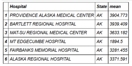
dplyr there is a function group_by() , and in data.table it is simply used by . head(hospital_spending_DT[,.(mean=mean(Avg.Spending.Per.Episode..Hospital.)),by=.(Hospital)]) mygroup= group_by(hospital_spending,Hospital) from_dplyr = summarize(mygroup,mean=mean(Avg.Spending.Per.Episode..Hospital.)) from_data_table=hospital_spending_DT[,.(mean=mean(Avg.Spending.Per.Episode..Hospital.)), by=.(Hospital)] compare(from_dplyr,from_data_table, allowAll=TRUE) TRUE sorted renamed rows dropped row names dropped attributes You can also use more than one grouping condition.
head(hospital_spending_DT[,.(mean=mean(Avg.Spending.Per.Episode..Hospital.)), by=.(Hospital,State)]) mygroup= group_by(hospital_spending,Hospital,State) from_dplyr = summarize(mygroup,mean=mean(Avg.Spending.Per.Episode..Hospital.)) from_data_table=hospital_spending_DT[,.(mean=mean(Avg.Spending.Per.Episode..Hospital.)), by=.(Hospital,State)] compare(from_dplyr,from_data_table, allowAll=TRUE) TRUE sorted renamed rows dropped row names dropped attributes Serial connection
Both
dplyr and data.table allow building chains of functions. In dplyr you can use pipelines from the magrittr package with %>% . %>% passes the result of one function as the first argument following it. In data.table , chaining uses %>% or [ . from_dplyr=hospital_spending%>%group_by(Hospital,State)%>%summarize(mean=mean(Avg.Spending.Per.Episode..Hospital.)) from_data_table=hospital_spending_DT[,.(mean=mean(Avg.Spending.Per.Episode..Hospital.)), by=.(Hospital,State)] compare(from_dplyr,from_data_table, allowAll=TRUE) TRUE sorted renamed rows dropped row names dropped attributes hospital_spending%>%group_by(State)%>%summarize(mean=mean(Avg.Spending.Per.Episode..Hospital.))%>% arrange(desc(mean))%>%head(10)%>% mutate(State = factor(State,levels = State[order(mean,decreasing =TRUE)]))%>% ggplot(aes(x=State,y=mean))+geom_bar(stat='identity',color='darkred',fill='skyblue')+ xlab("")+ggtitle('Average Spending Per Episode by State')+ ylab('Average')+ coord_cartesian(ylim = c(3800, 4000)) Average costs per case by state
hospital_spending_DT[,.(mean=mean(Avg.Spending.Per.Episode..Hospital.)), by=.(State)][order(-mean)][1:10]%>% mutate(State = factor(State,levels = State[order(mean,decreasing =TRUE)]))%>% ggplot(aes(x=State,y=mean))+geom_bar(stat='identity',color='darkred',fill='skyblue')+ xlab("")+ggtitle('Average Spending Per Episode by State')+ ylab('Average')+ coord_cartesian(ylim = c(3800, 4000)) Average costs per case by state
Conclusion
We looked at how you can perform the same operations using the
data.table and dplyr . Each package has its advantages.The code used in this article is available on GitHub .
Source: https://habr.com/ru/post/302624/
All Articles