About the three-dimensional Z-order put in a word

“Once upon a time, it seems, last Friday,” the author was struck by an article that compared various popular methods of indexing celestial objects. Due to uneven breathing, this topic had to be understood in its intricacies and draw conclusions.

You ask: “Who cares about these celestial objects?” And even: “Well, what does 2GIS have to do with it?” And you will be partly right. After all, spatial indexing methods are universal value.

Usually, when dealing with geodata, we work with a local projection onto a plane and thereby dismiss distortion. On the scale of the planet, it is more difficult to do this - astronomical problems begin to bulge.
As for data volumes, now in OSM there are more than 4 billion points and 300 million roads. This is commensurate with the scale characteristic of stellar objects. And among other things, star atlases are an excellent stand for developing and debugging spatial algorithms.
')
The promised subtleties and conclusions under the cut.

Prelude

The problems of indexing celestial objects is a struggle against polar coordinates.
Since objects traditionally have the coordinates RA / DEC (latitude / longitude), the length of the degree of longitude depends on the latitude, and singularities appear at the poles. Therefore, when searching in the vicinity of a certain point, it is necessary to take into account the latitude of this point when building the search extent. And I would like to hide these details inside the index.
In the case of a spatial join, again, I do not want to load the SQL processor with various intimate details.

So, the main external requirements for the indexing method ("pixelization") of celestial objects are as follows :

1. Hierarchical structure.
2. Equal areas. This means that the area under the “elementary pixel” should not (ideally) depend on the latitude and longitude.
3. Isolatal distribution of data. A good indexing method leads to the fact that at any latitude on the "elementary pixel", on average, there are the same number of objects. For geo-objects this is not the case, by the way.

Of course, the use of a DBMS imposes its own limitations: the “pixel” number should be easily calculated, the index should be compact, the search query should generate a moderate number of subqueries.

There are quite a few spherical polyhedra , related methods ( HEALPix , HTM ). It is possible, moreover, to undertake the paving of the sphere by such a method here (or by a similar):

(The correct heptagonal parquet of order 3 in the Poincare model on the disk )
But the one who comes up with a cheap way to translate the coordinates into a pixel number for this variant and get a set of pixels along the cone risks invoking the devil.

Let's get started

The article mentioned compares various popular indexing methods implemented in Postgres.

1. HAVERSINE - the DEC (declination, longitude) field is indexed, then the data is filtered;
2. UNIT VECTOR - the DEC field is indexed; during filtering, the scalar product of the vector of the test point and the axis of the request cone is calculated. The cosine of the deviation must not be less than the specified (cone query);
   
3. POSTGIS - r-tree in RA (right ascension, latitude) / DEC coordinates;
4. Q3C -
   
   • when indexing
     
     1. the points are projected on the faces of the cube,
     2. the number of the face falls into the high bits (3 bits for 6 faces) of the index value,
     3. The low -order bits are encoded using a Z-order , which turns the coordinates on the face,
     4. for a 32-bit value, the maximum depth level is 14 (14 * 2 + 3 = 31). For a 64-bit value, a depth of 30 is available, but in fact 16 (see the constant Q3C_INTERLEAVED_NBITS),
        
     5. the calculated values ​​are placed in a regular B-tree;
   • when searching
     
     1. the cone of inquiry is projected on the verge lip and forms an ellipse,
     2. at worst (angle) it can be three ellipses and three subqueries,
     3. the ellipse is rasterized on the face lattice, the result is a list of pixels covered by it,
     4. the pixels are translated into a Z-order and thus a list of index intervals is obtained, potentially containing the necessary data,
     5. then the search by index and (possibly) finer filtering takes place;
   • pros
     
     1. simplicity
     2. regular compact index
     3. relatively small unequal pixel areas,
     4. high search speed on small queries;
   • minuses
     
     1. it is still a block index. The maximum index depth is 16 bits + 2 bits on 4 faces at the equator. In 2MASS, the resolution of the telescope is the fractions of angular seconds, even 0.5. We have 2 * 60 * 60 * 360 = ~ 2 ** 21,
     2. The index is intended for small queries. Otherwise, the ellipse will cover a large number of intervals of the index and this will become a problem, because at this moment we do not know which of them are not empty, we’ll have to check everything. However, this is not a Z-order problem, the index with the lower-case scan would behave no better. This problem is caused by the fact that we have no idea from the outside how the tree is actually (filled). On the other hand, this deficiency is compensated for by the blockiness of the index, perhaps, problematic in size queries rarely occur in astronomy,
     3. The two moments described balance each other. We cannot just take and increase the resolution of the index, as there will be an explosion in the number of intervals. And we cannot reduce it, since the load on post-filtering will increase due to the coarseness of pixels;
5. PGSPHERE - the points are placed on a sphere of unit radius and their three-dimensional coordinates are indexed in the r-tree.
   
   • pros
     
     1. great idea,
     2. exact index, it does not require post-filtering,
     3. staff index for the database;
   • minuses
     
     1. r-tree is quite “thick”, rating : 4 times,
     2. and, therefore, page cache efficiency drops,
     3. the behavior of the r-tree is highly dependent on page splitting heuristics, for such specific data it would be good to choose the optimal heuristics,
     4. Depending on the chosen heuristic, the r-tree may begin to degrade if the data changes intensively, for a B-tree, by the way, such degradation does not occur.

Actually, the results

Details of the comparison:

• the first 2 columns - search (first and subsequent) in HEASARC dataset (36,000,000 lines) with an accuracy of 1 degree, used a series of 162 search points;
• 3 and 4 columns - spatial join (with a radius of 0.01 degrees) between Swift (76.301 lines) and XMM (2,880,728 lines), the first and subsequent runs.

The relative results are as follows:

What should I look for?

1. PGSphere is far ahead of all other methods in the search. Potentially, Q3C could be faster than PGSphere, but apparently, the shortcomings of high-level Z-order are already beginning to manifest themselves on requests with a radius of 1 degree, the number of subintervals is too large.
2. PGSphere is faster than PostGIS, although a more complex three-dimensional tree is used. This can be explained by the struggle with distortions at the poles, which do not allow to use the index at full power.
3. PGSphere is slower in Q3C in spatial join'e twice. What are the explanations?
   
   1. Spatial join - a series of searches with small radii, where search queries are taken from the master table (Swift) and performed on the slave (XMM).
   2. In this case, the request radius is significantly less - 0.01 degrees. At this radius, all the advantages of the Z-order are preserved and its drawbacks do not yet appear.
   3. The PGSphere slowdown is most likely caused by a less efficient page cache.
4. Q3C at least twice as fast as PostGIS.

It's time to ask a question from the category of "what if ...".

What if?

If you make a hybrid PGSphere and Q3C, where instead of the R-tree uses a three-dimensional low-level Z-order. Why Z-order, what's good about it? At a minimum, this indexing method automatically satisfies the three primary external requirements that are formulated at the beginning of the article. There are "internal" advantages.

Z-order

One of the most famous examples of a self-similar curve sweeping a square is the Hilbert curve . Another slightly less well-known example is z-order .
Our order of detour is somewhat different from the canonical, but it does not matter.
Each pair of x-bit numbers (x, y) is assigned a 2x-bit z by the following simple rule. Bits of numbers x, y are connected into one number, just alternating with each other. In this case, the bits of the number x occupy even positions (if one starts counting from 0), and the bits of the number y are odd.

For a 64x64 square, it looks like this:

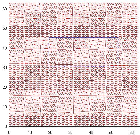
Z-order is very useful for indexing, as it can be implemented as a regular B-tree with an integer key. However, there are problems with effective search for it.

The blue box in the picture is a search query. Each time it crosses a curve, a continuous interval of key values ​​is generated (or ends).
Therefore, if we process each such interval in a separate subquery, we get significant overhead, since a large part of these intervals are empty, and each subquery is a passage through the index tree.

If we search in one interval from the beginning to the end of the extent, this is equivalent to as if we indexed one Y-coordinate and filtered it. To query 1/10 from the extent of the layer by x & y (1/100 of the layer) it will be viewed 1/10 of the index - Efficiency 10%, for a request to 1/100 of the extent of the layer by x & y (1/10000 of the layer) 1/100 of the index will be viewed - Efficiency 1%.

This explains why this method is rarely used in a DBMS. So in Q3C it is in block version. Although self-similarity gives it a wonderful feature - adaptation to unevenly distributed data. In addition, continuous segments of the curve can cover large areas of space, which is useful if you are able to use it.
There is an effective (but very low-level) way to work with Z-order, but more on that, perhaps later. This method also applies to the three-dimensional index.

However, the behavior of Z-order in three-dimensional space is poorly understood and requires careful verification. What we do.

Z-order in 3D

What do we want to see?
How do you generally evaluate the suitability of the indexing method for processing spatial data?

As already mentioned , no matter what we do, the index file on the physical medium (pagination) is one-dimensional, and it is impossible to arrange two (multi) dimensional data without gaps.
Self-similar curves give us the ability to minimally observe the locality of the links, that is, spatially close objects and on the disk will often be close. The most pleasant in this respect is the Hilbert curve, but it is expensive from a computational point of view. Z-order is just a compromise between the requirements for computational simplicity and data locality.
But still very often close points will be far from each other. How to evaluate the degree of "imperfection" of indexation?

First , we will proceed from the fact that the spatial index is located on the pages of the tree. And if two points hit one page, then they are physically close, even if the corresponding Z-values ​​are very different.
Secondly , spatial search is performed in a certain extent, therefore, the smaller the number of pages that fall into this extent, the higher the request processing speed.
Thirdly , if the search query is smaller than the typical page size, the index is “better”, the more likely it is that the search will be limited to one page.

So, we can formulate a general rule:
A “good” indexing method minimizes the total perimeter of index pages .
It would be worthwhile to come up with a formal criterion for assessing quality, but sometimes it is better to see everything once with your eyes than to juggle with numbers. And getting a general understanding of the situation can be addressed and formalization.

Numerical experiment

In order to fit in 64 bits, we allow a resolution of 21 bits for the original coordinates.

For the first series we will place on the upper hemisphere of a unit radius a point with a step of half a degree in latitude and longitude.
The central part of the hemisphere looks like this (in the order of generation, the gnuplot command: 'splot' data 'wl;'):


Now we will build Z-values ​​for each point and sort them according to these values. Values ​​are planted on the grid in the intervals of 0 ... 2 000 000 (ie, 21 bits). For control, we will also build a picture for a 2-dimensional z-order (only x & y, without z).

Fragment 3d, a general view of the crawl from above. In addition to the "lumbago" (from transitions through the degree of 2-ki) along x & y are also visible annular "lumbago" in z.


Same for 2d.

Now we will simulate the distribution of data on pages on the disk. Suppose 1000 elements fall on a page. Then the first 1000 elements in the sorted array will go to the first page, etc. For clarity, presented bypassing the page, but it is not important - as we have already found out, the perimeter is important.

The first 1000 values.

Values ​​from 9000 to 10,000.

Values ​​from 19,000 to 20,000.

The values ​​are from 60000 to 61000. Since the sphere in this place has practically expanded, 2d and 3d coincide.

Values ​​from 120,000 to 121,000. Hit the node.

Now we prepare 150,000 random points on the sphere and do the same with them.
A general view of the bypass on top is now this:

The polar region does not stand out, and it pleases.

It is almost the same for both cases.

The first 1000 values.

Values ​​from 9000 to 10,000.

Values ​​from 19,000 to 20,000.

Values ​​from 60,000 to 61,000.

Values ​​are from 120,000 to 121,000.

findings

1. As expected, the pseudo-three-dimensional (on the sphere) spatial index, based on the sweeping curve, behaves very much like its two-dimensional version.
2. It is still easy to calculate.
3. The index itself is implemented in the form of a tree structure, which is very convenient for a DBMS.
4. It has all the necessary qualities for indexing celestial objects.

However, apart from the merits, he also has all the flaws of his two-dimensional version, and in a hypertrophied form. If we try to look in the index in the forehead, looking for continuous intervals of values, we will be disappointed, these intervals have become even more. In essence, head-on can only be searched in very small extents.

As already mentioned, there is a method for working with such an index. But that's another story.

PS

I would like to express special thanks to Sasha Artyushin from DataEast for conceptual participation.