New derivatives of Bessel functions are derived using the Wolfram Language.

Almost two hundred years after Bessel introduced his functions of the same name, expressions were found for their derivatives with respect to parameters, valid in the entire complex plane.

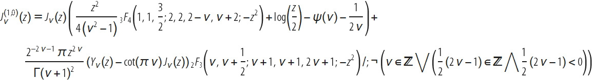
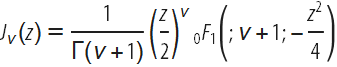
In this blog, we present and comment on some previously unknown derivatives of special functions (first of all, Bessel functions and related functions), as well as touch on the history and current state of differentiation by parameters of hypergeometric and other functions. One of the main new formulas (in more detail below) is the closed expression for the first derivative of one of the most popular special functions — the Bessel function J :



Many functions of mathematical physics (that is, functions that are often used and therefore have special names) depend on several variables. One of them, as a rule, is called an argument, while the others, as a rule, are called parameters or sometimes indices (icons). These special functions can have any number of parameters. For example (see Wolfram Functions Site ), Bessel functions (z) and (z), Neumann (z) Macdonald (z) and Struve (z) and (z) have only one parameter (the so-called index), while the Whittaker functions (z) and (z), as well as degenerate hypergeometric functions (a; b; z) and U (a, b, z) have two parameters. Anger functions (z) and (z) as well as Weber functions (z) and (z) can have one or two parameters (in the case of two parameters, they are called the generalized functions of Anger and Weber). The Appell and Humbert functions have from three to five parameters, while more complex special functions, such as the generalized hypergeometric function may have any finite number of parameters.
')
Among other properties, the differentiation of special functions plays a significant role, since derivatives characterize the behavior of functions as these variables change, and they are also important for studying the differential equations of these functions. As a rule, the differentiation of a special function by its argument does not present significant difficulties. The largest collection of such derivatives, including first, second, symbolic, and even fractional order for more than 200 functions, is available in the “Differentiation” section on Wolfram Functions (for example, this section includes expressions for the 21 derivative Bessel functions (z)), or in the book of Yu. A. Brychkova Handbook of Special Functions ). Most of these formulas are also available directly in the Wolfram Language . They can be obtained using the new Mathematical FunctionData and EntityValue functions .

However, derivatives with respect to parameters (as opposed to an argument) are generally more difficult to compute. It is noteworthy that the above formula, which includes a first order derivative (with respect to the parameter ν ) of one of the most frequently encountered special functions of mathematical physics, has only recently been found in a closed form, and this surprising fact may indicate the complexity of the general problem. Thus, using the Bessel function J as a typical example, we will take a brief tour of the history of the differentiation of this special function.

Calculating derivatives is not always easy.

Often, people who are even familiar with mathematical analysis tend to think that it is difficult to integrate, and it is easy to differentiate. The “popular” wisdom is well known, which says that “ differentiation is a matter of technology, and integration is an art ”. But this statement is fully true only for elementary functions, for which differentiation leads again to elementary functions (or their combinations). If differentiation is carried out by parameters, it, as a rule, leads to complex functions of a more general class.

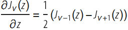
The difference between differentiation by parameters and differentiation by argument can be illustrated by the Bessel function J. Bessel’s J derivative in its argument z has been known for quite some time and has a relatively simple closed form:



However, analytical calculation of its derivative with respect to the parameter ν is more complicated. Often, derivatives with respect to parameters can be written as an integral or an infinite series, but these objects cannot be represented in closed form through other simple or known functions. Historically, some special functions were introduced for the sole purpose of giving a simple notation for derivatives of known functions. For example, a polygamma function originated as a means to represent derivatives of a gamma function .

Generalized hypergeometric function and its derivatives play an essential role in solving various problems of theoretical and applied mathematics (see, for example, the article by LU Ancarani and G. Gasaneo regarding the use of derivatives with respect to parameters in quantum mechanics). The generalized hypergeometric function generates as special cases many of the most frequently used elementary functions (for example, trigonometric, hyperbolic, logarithmic, and inverse trigonometric functions), as well as many special functions, including the Bessel, Struve, Kelvin, Unger-Weber, incomplete gamma function and integral functions (exponential, sine and cosine). In case p = 0 , q = 1 , the generalized hypergeometric function contains the Bessel family of functions (z) (z) (z), and (z) The Bessel function J , for example, has the following hypergeometric representation:







It is interesting that the history of the function (z) begins almost exactly 200 years ago. In the reports of the Berlin Academy for 1816–17 (published in 1819), in the paper Analytische Auflösung der Keplerschen Aufgabe , Friedrich Wilhelm Bessel considers the so-called Kepler equation M = Ee sin (E), where M is the mean anomaly, E is the eccentric anomaly, and e - eccentricity of the Keplerian orbit. The solution of this equation can be represented (in the modern notation) through Bessel functions of integer order:



In this first work, Bessel still does not use modern notation, but its function appears already in an implicit form. For example, he uses the following amount (note that Bessel uses the Gauss designation for i ! ):



Nowadays, we can write this expression as the sum of two Bessel functions in the Wolfram Language as follows:





This sum is just the first derivative of the Bessel function -2 ae (ei):





In his next work in 1824, Bessel uses almost modern notation (replacement J I ) to designate his function:







It also displays the fundamental relations for this function, such as:







Various special cases of the general Bessel function are already found in the writings of Bernoulli, Euler, D'Alembert, and others (for more, see the article ). The main reference book on Bessel functions to this day remains the classical monograph by G. N. Watson “ The Theory of Bessel Functions ”, which was reprinted many times and was significantly supplemented in comparison with the first edition of 1922.

Thus, while the derivatives of the Bessel functions J with respect to the argument z have been known since the beginning of the nineteenth century, it was not until the middle of the twentieth century that particular cases were found for index derivatives. The derivatives of some Bessel functions with respect to ν at the points ν = 0, 1, 2, ... and ν = 1/2 were given by J. R. Airy in 1935, and expressions for other functions of the Bessel family at these points were given in the book of V. Magnus , F. Bateman and R. P. Soni “ Formulas and theorems for special functions of mathematical physics ” (1966):



A generalization to any half-integer values ​​of ν was presented at the International Conference on Abstract and Applied Analysis (Hanoi, 2002) as follows:



These results, along with expressions for derivatives with respect to the parameter of the Struve functions in integer and half-integer points, were published in 2004–2005. Various new formulas for differentiating Anger and Weber functions, Kelvin functions, incomplete gamma functions, parabolic cylinder functions, Legendre and Gauss functions, generalized and degenerate hypergeometric functions can be found in the “ Special Functions Guide: Derivatives, Integrals, Series, and Other formulas . For a quick overview and links, see H. Cohl .

Probably, it seems surprising that in the presence of all these results, the first derivatives of Bessel functions in closed form with arbitrary parameter values ​​were obtained only in 2015 (Yu. A. Brychkov, “ Higher derivatives of Bessel functions with respect to the index, ” 2016) . They are expressed as combinations of products of Bessel functions and generalized hypergeometric functions. For example:



The graphs below give some insight into the behavior of the Bessel function. (z) and its derivative in areas of interest. First, we give (in real ν - z -planes) an expression for the first derivative of (z) by ν (see the equation at the beginning of the article):





For a fixed index, namely ν = π , we present the graphs of the Bessel function along with its first two derivatives (in argument and index):





It is interesting to note that the derivatives (with respect to z and with respect to ν ) have almost identical zeros.

How did we get it?

It is noteworthy that even almost 300 years after the introduction of the classical function (the Bessel function (z) was introduced by Daniel Bernoulli in 1732), you can still find new and relatively simple formulas related to such functions. In fact, the formula for the derivative introduced above (along with the corresponding results for the derivative , and the functions of Neumann, MacDonald and Kelvin) were obtained using the Wolfram Language. Details on how these derivatives were sought are published here . In this post, we present only a sketch of one of the variants of the approach that can be used for other special functions.

First, we recall that the Bessel functions and the others we are interested in are functions of a hypergeometric type; but differentiation by parameters of a common hypergeometric function of one variable requires more complex hypergeometric functions of more than one variable (see LU Ancarani and G. Gasaneo). First derivative with respect to “upper” parameters , and all derivatives of symbolic integer order m with respect to the “lower” parameters generalized hypergeometric function can be expressed in terms of Campe de Ferrier hypergeometric function two variables according to the following formulas:





The above Campe de Ferrier hypergeometric function is defined by a double row (see here and here ):



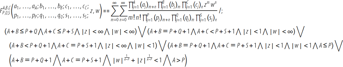
The Campe de Ferrier function can be considered as a generalization of a hypergeometric function into two variables:



The corresponding regularized version of the function can also be determined by replacing the product of Pohgammer symbols in denominator on .

The Campe de Ferrier function can be used to represent the derivatives of the Bessel function J by parameter:



This expression coincides with the simple formula above, which includes hypergeometric functions of one variable, although this is not immediately obvious (we still do not have a complete set of formulas to simplify multidimensional hypergeometric functions to expressions containing only one-dimensional hypergeometric functions).

Double series, similar to the above definition of the generalized hypergeometric function of two variables, also arise when calculating the Mellin transform from the products of three Meyer G-functions :



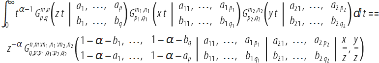
The right-hand side of this formula includes the Meier G-function of two variables, which in the general (non-logarithmic) case can be represented as a finite sum of Campe de Ferrier hypergeometric functions with some coefficients, by analogy with two formulas ( first , second ) for G- Meyer functions are one variable. Finally, the Campe de Ferrier function also arises when the real and imaginary parts of hypergeometric functions are separated from one variable, z = x + iy , with real parameters:


(The above formula was derived by E. D. Krupnikov, but not published).

It should be noted that in recent years, hypergeometric functions of many variables are finding an increasing number of applications in such fields as quantum field theory, chemistry, mechanical engineering, communication theory and radiolocation. Many practical results can be presented using such functions, and therefore most of the main results in this area are obtained in the applied scientific literature. The theory of such functions in theoretical mathematics is still relatively poorly developed.

Symbolic derivatives in the Wolfram Language

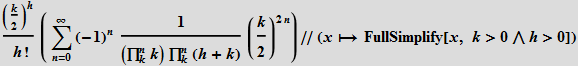
The author of these new and interesting formulas with symbolic derivatives, Yuri Brychkov, is a member of our team, which allows us to bring this constantly developing area of ​​mathematics to the attention of our users. We are also lucky that we have at our disposal a new feature of Mathematica (Wolfram Language) - Entity , which allows, among other things, to quickly (within a few weeks or days) present new results in a calculated format and on all platforms that use the language Wolfram Language, our users. For example, in the Mathematica system, the following expression can be calculated:





Thus, we get the basic formula of this article. We can test the formula numerically, first substituting the symbolic values ​​of ν and z , and obtaining the expression:





Next, we separate the left and right sides and substitute random values ​​for the argument and parameter:





The numerical derivative of the left side is calculated in the Wolfram Language using a limit procedure. The equality of the left and right sides, and therefore the correctness of the initial formula for the derivative, is obvious.

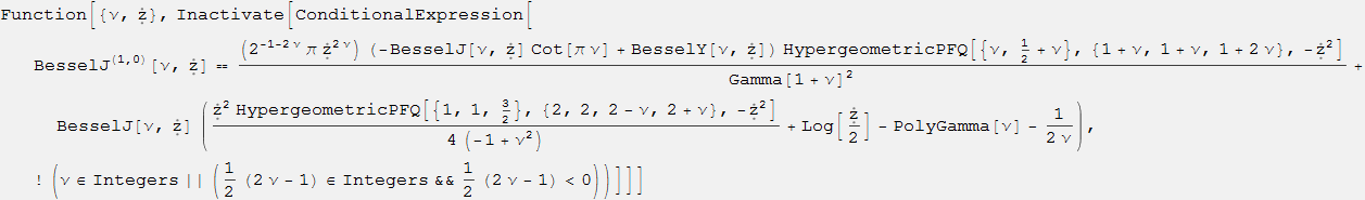
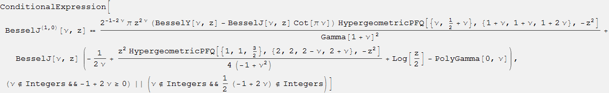
In addition to many new results on symbolic and parametric derivatives, which were mentioned in this article and are only available through EntityValue (although deeper integration of this functionality in future versions of the Wolfram Language requires constant effort), a large number of results in this area have already been implemented into the core of the system. Mathematica and the core of the Wolfram Language. Such parameter derivatives are not calculated automatically because of their complexity, but they can be seen using the FunctionExpand command. For example:









Derivatives on the index of the second and higher order Bessel functions and related functions can be expressed in terms of the Kampe de Ferrier hypergeometric function of two variables , but the resulting formulas can be quite complex, and can include Bell's Y polynomials:



The last expression arises from the Bessel function representation. (z) through function composition (; ν + 1; w) and :



We use the Faa-di-Bruno formula , which allows us to obtain the expression for the nth derivative of the composition of m functions . In the case of m = 2 (see here and here ), we get, for example, the expression:



The corresponding formula for common m and n can be obtained and verified in the Wolfram Language:





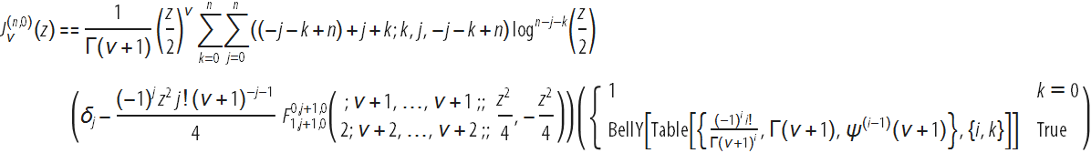
While Bell's Y polynomials, for which there is no generic closed form, are usually necessary to represent higher order derivatives, one of the authors of this post, Yuri Brychkov, found a way to eliminate Y polynomials from the nth derivatives on the parameter of Bessel functions, leaving us with a wonderful result:



For the convenience of interested users who would like to see in one place all known formulas for derivatives of special functions on parameters (including those listed above), we collected and presented these formulas in the following ways:

1. In tabular format (download here ).

2. Mathematica laptop format (download here ).

3. A subset of the formulas that were known before 2009 can be seen on the Wolfram Function Site website in the “Differentiation” sections of various functions (for example, see this page ).

In our next post we will give expressions of a closed kind of derivatives for a collection of more than 400 functions with general rules for derivatives of symbolic and fractional order. We hope you enjoy exploring the world of special-purpose derivatives using the Wolfram Language!

For questions about Wolfram technologies, write to info-russia@wolfram.com