Node-SPICE: Simulation of transients in the electrical network
Hello! Today I want to talk about one of his projects, which was created as one of the tools for obtaining data for the thesis, and since at the moment he has completed his main task, I want to put him into the GPLv3-swimming - maybe it will be useful to someone still. However, before giving the moorings, I decided to use the Intel Vtune Amplifier profiler to make sure that my simulation package for the tree-like power supply network optimally consumes the computing resources of the computer.

Under the cut, details about myself, about the project and about performance optimization (which we managed to increase more than twice in half an hour)
For the last 6 years I have been working on issues of energy saving and improving the quality of electricity at industrial facilities. First of all, it is compensation of reactive power at the level of the consumer of the electric power, so that this most reactive power is not consumed from the industrial network of power supply. Parallel to this task is the task of stabilizing the voltage in the nodes of loads, directly next to consumers.
')
Imagine a conventional asynchronous motor. Thousands of them. Look like this:
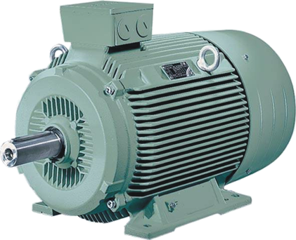
In various authoritative and not very sources, one can find statistical information that up to 70% of the generated electricity is consumed by asynchronous electric motors. I do not think that the real figure is far from this value.
So, have you ever noticed that if the old refrigerator starts at home, the light blinks? This effect - flicker - occurs due to the fact that when starting the motor consumes current 5-7 times more than the nominal. At the very first moments of start-up, there is no magnetization of the stator, the inductive resistance is minimal and the network is actually loaded with a rather small active resistance of the stator winding. Then, when the engine starts to gain momentum, the stator magnetizes, the reactance of the stator winding increases and the current decreases.
Now imagine the electrical network of the enterprise:

Fig. 1 - Main power circuits for power consumers: a - with distributed loads; b - with concentrated loads; in - block transformer - highway; 1 - substation switchboard; 2 - power distribution point; 3 - electric receiver; 4 - highway; 5 - tire assembly.
This is such a tree-shaped branched electrical network with many electrical receivers. In general, you can draw it like this:
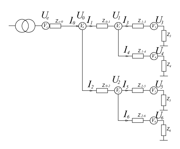
Fig. 2 - Generalized block diagram of power consumers.
In the diagram in fig. 2, the Ve node is the connection point of the power supply network (industrial AC network, ship generator, wind generator inverter, etc.), as a result of which the node voltage becomes Ue . To the source by means of an active-inductive supply line with resistance Ze = Re + jLe , a distribution node V0 is connected with a voltage U0 , which is defined as:

where I_ {e-0} is the current consumed from the node Ve , which is equal to the sum of the currents consumed by the subordinate loads:

where N is the number of loads powered from a given node. For the diagram in fig. 2 from the Ve node, all the load nodes in the system are powered - V3 - V6 . Node-loads V3, V4 are connected to node V1 ; and to node V2 nodes-loads V5, V6, respectively.
If one of the loads changes, the current changes in the whole circuit to the root, therefore, the voltage changes in the root, and behind it in all other nodes. And if we need to stabilize the voltage at several points in the circuit, then the problem arises of doing it optimally, because the two stabilizers will influence each other. To trace this effect on a variety of options, it is necessary to perform network simulation.
The diagram in fig. 2 You can draw yourself in the Matlab Simulink package. But there is one snag - if the scheme is large, or there are many of these schemes, then draw each scheme, run the simulation, remove and save the simulation results, transient graphs, damn dreary, and I decided that it would be faster to create my own modeler (fig) and more interesting (and here I was right).
In order for the development to be even more interesting and useful, I, a severe Sishnik-piece of iron, decided to deal with C ++ as the development language at last.
The sources are a Visual Studio 2013 project and are uploaded to GitHub .
To build the application, you need to download the Eigen linear algebra library and specify the path to the library folder using the system environment variable $ (EIGEN_DIR) . Visual Studio will have to pick up the path to this folder and compile the application without any special rustling.
To output and save graphs, the application uses the gnuplot package with the cairo module - gnuplot should be able to save images in PNG format. You can verify this by running the set terminal png command in the gnuplot console. Gnuplot should not swear at the wrong argument - gnuplot, which comes with octave, was the last one to sin. The path to gnuplot must be in $ (PATH) .
The application was supposed to consist of modules independent of each other (Figure 3), but something went wrong:
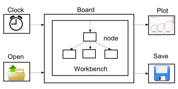
Fig. 3 - Program flow chart
The main modules of the system are:
The interface of the program console - the types and parameters of power consumers, as well as the configuration of the load node are described in configuration files.
The startup command looks like this:
The format of the configuration file is text, consisting of lines of the form:
where a, b, c, d, e are parameter keys, some of which (a, b) have a boolean data type - active or inactive option or mode. The other part, for example, c, d, e, has a textual or numeric value of the parameter.
A configuration file in which a three-phase voltage source is connected via a quality analyzer to an electric motor and an unbalanced load is as follows:
On the Workbench desktop, there can be any number of elementary Node nodes connected in a tree-like configuration.
Each node has an input for connecting a voltage source and an output for powering a subsequent load. To the output of one node can be connected to the inputs of several child nodes. The parent node sets the voltage at the terminals of the child node and requests the current consumed by it. If the child node has its own child nodes, then the operation is performed recursively. The behavior of the node is different - the voltage source, which is unique in the system. After the simulation stage, the source is provided with information about the total current consumption and returns information about the current value of the voltage at the source output.

Regardless of their type of nodes have a common interface that allows you to create different hardware configurations. The elementary node is added using the load command.
General view of the load command:
There are the following configuration keys common to all nodes:
Implemented types of elementary Node nodes:
It is assumed that each desktop is a kind of scheme and it should be possible to create nested schemes, i.e. nested desktops. This feature is incorporated in the test version of the program (but, of course, not implemented :)). Unique keys for the desktop are missing. Since there may be several desktops, after the introduction of a second or more desktop for nodes, you should specify which desktop they belong to. If the -wb switch is not specified, then the elementary node will be placed on the last created desktop.
In the current version of the software package there can be only one voltage source, which somewhat limits the capabilities of the program, but is sufficient for my task.
I have little thoughts to take everything and rewrite, using a complex calculus, any number of sources and receivers of electricity of any configuration, but I tearfully implore myself if I sit down for it, then AFTER a thesis. While holding on.
Figure 5 shows the process of modeling a voltage source without load:

Fig. 5 - Graphs of current and voltage of the voltage source operating in idle mode
The consumption quality analyzer is included in any part of the system and analyzes various parameters of consumption. This node is responsible for the construction of graphs.
After the simulation, the node using the Plot module displays the required graphs and saves them to disk as images.
This elementary node implements a mathematical model of an asynchronous electric motor.
Figure 6 shows the process of starting an asynchronous motor. At time 1 s. A torque of 700 N * m is applied to the shaft and the engine goes into operating mode.
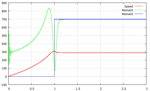
Fig. 6 - Graphs of the frequency of rotation of the motor shaft, as well as the torque on the shaft and the static torque when the engine is started
This elementary node is a parallel connection of active resistance, inductance and capacitance. Depending on the parameters, it allows modeling the following standard and non-standard modes of exposure to a voltage source: one- and two-phase load, asymmetrical load, short circuit in phase short and long in time, short circuit to earth in all phases, short and long in time.
Simulate short-term short circuit in the network:
KZ 0.1 s. The speed does not have time to fall below the critical, the engine restores speed after removing the short circuit.

CZ 0.5 s, the engine has time to brake and after switching on the engine torque becomes less than the torque on the shaft and the engine crashes
The closure in Phase A. The speed practically does not sag, because of the peculiarities of the asynchronous electric motor, it only needs two phases. The rotating magnetic field in the gap takes an oval shape and the shaft begins to vibrate with the frequency of the supply network.
In general, as it turned out, the main process of modeling itself was written quite accurately and no architectural changes were made according to the results of the modeling. But the devil is in the details.
Open Intel Vtune Amplifier, create a new project:
Specify the path to our program and launch keys. It would be nice to use the Binary / Symbol Search and Source Search buttons and specify the paths to the source code and binaries with Debud-symbols - then it will be more convenient to navigate through the project and the source code.
We use the following config:
All the above config files are in the / doc folder of the project.
Let's start with the simplest basic hotspot with an interval of 1ms

And run.
Top Hotspots:
Holy neutrons ... Of course, I knew that iostream is slow, but so much ... This, by the way, is disabling synchronization with
20 seconds of CPU time out of a total of 35 seconds. More than 50% of the time. It does not go into any gate.
You can read more about how slow the threads are here . It makes sense to rewrite everything to armored fprintf (). I was also interested that the cout function appears in the table twice. And for sure - the gnuplot layer creates temporary files and then deletes them. Add the -raw key to the node to save the raw graph files. There are keys - saved, no, not saved.
Run the profiler. Ha!
Top Hotspots:
The leaders are still file output, but consuming less than 5% of CPU time. Serious success! Watch Bottom-Up three
The second and third place is taken by pointers and iterators:
And that is quite logical - the place gets the power quality analyzer, because the latter does a lot of all the work.
This code was written as a test of the concept of sliding measurement mode. As can be seen from the code, each new step of the solver is associated with a shift of a small (64-128 characters), but still an array. It makes sense to use a ring buffer to solve this problem. Then the operation of adding a new element will have the value O (1) instead of O (N).
“Why is this necessary?” You say, they say, the quality analyzer is one in the system, it is better to add motors to the config. And you will be half right - we will definitely add the motors, only analyzers in the system can be exactly as much as in the system of nodes - this is a feature of my thesis.
Let's look at what’s wrong with GetVoltage and GetCurrent bad:

Hmm, how about using links?
Restart profiling:
Top Hotspots:
Bottom-Up three shows that, again, the first in the list is our fprintf and pango, crawling out from under the gnuplot - we’ll no longer be crawling into them (although it would be worth it).
What really pleases is the fact that NewStep, from which a couple of steps to Solve took the lead. Run the simulation for 40 seconds and see how the picture changes:
The effect is scaled, so here we have nothing to do.
Summarize
Not bad for half an hour of work?
Add to the engine heel system:
From Bottom-Up three, little is clear:

Now, if you look at the Caller counter, you can see where the resources go. On the solution of matrix equations in the calculation of mat. motor models - most of the time the Eigen library is running.
We won’t get into the library; we’ll better replace the motors with rl-loads. They are much more important to me - you can create all sorts of different phase distortions, short circuits, disturbances and other joys.
Since we don’t really need to count anything on one tick, we’ll increase the clocking frequency of the solver, and we will increase the loads to 10 units.
Fprintf we do not touch, but the main culprit:
Here we copy the double [4] vectors into each other. As you can see, vector copying by means of the vector itself is not very optimal. Zababahay we ka cycle - for 4 elements, especially it is not necessary to run out:

And the last time

And they do not have. I decided for myself that it was useless to upload brake applications in OpenSource and sat a little with a convenient and powerful profiling tool. In contrast to the placement of timestamps inside the code, Vtune, as they say, “pokes the muzzle” into a slow code, hinting that it would be nice to rewrite one or another piece.
My application, in fact, can be infinitely optimized - for a crutch on a crutch. You can throw out Eigen and rewrite Acmotor using Boost; you can write graph output on the same Boost; .
By the way, here you can get a free version of Intel parallel Studio for student and educational needs.
Under the cut, details about myself, about the project and about performance optimization (which we managed to increase more than twice in half an hour)
Introduction
For the last 6 years I have been working on issues of energy saving and improving the quality of electricity at industrial facilities. First of all, it is compensation of reactive power at the level of the consumer of the electric power, so that this most reactive power is not consumed from the industrial network of power supply. Parallel to this task is the task of stabilizing the voltage in the nodes of loads, directly next to consumers.
')
Imagine a conventional asynchronous motor. Thousands of them. Look like this:
In various authoritative and not very sources, one can find statistical information that up to 70% of the generated electricity is consumed by asynchronous electric motors. I do not think that the real figure is far from this value.
So, have you ever noticed that if the old refrigerator starts at home, the light blinks? This effect - flicker - occurs due to the fact that when starting the motor consumes current 5-7 times more than the nominal. At the very first moments of start-up, there is no magnetization of the stator, the inductive resistance is minimal and the network is actually loaded with a rather small active resistance of the stator winding. Then, when the engine starts to gain momentum, the stator magnetizes, the reactance of the stator winding increases and the current decreases.
Now imagine the electrical network of the enterprise:
Fig. 1 - Main power circuits for power consumers: a - with distributed loads; b - with concentrated loads; in - block transformer - highway; 1 - substation switchboard; 2 - power distribution point; 3 - electric receiver; 4 - highway; 5 - tire assembly.
This is such a tree-shaped branched electrical network with many electrical receivers. In general, you can draw it like this:
Fig. 2 - Generalized block diagram of power consumers.
In the diagram in fig. 2, the Ve node is the connection point of the power supply network (industrial AC network, ship generator, wind generator inverter, etc.), as a result of which the node voltage becomes Ue . To the source by means of an active-inductive supply line with resistance Ze = Re + jLe , a distribution node V0 is connected with a voltage U0 , which is defined as:
where I_ {e-0} is the current consumed from the node Ve , which is equal to the sum of the currents consumed by the subordinate loads:
where N is the number of loads powered from a given node. For the diagram in fig. 2 from the Ve node, all the load nodes in the system are powered - V3 - V6 . Node-loads V3, V4 are connected to node V1 ; and to node V2 nodes-loads V5, V6, respectively.
Why was Node-SPICE created?
If one of the loads changes, the current changes in the whole circuit to the root, therefore, the voltage changes in the root, and behind it in all other nodes. And if we need to stabilize the voltage at several points in the circuit, then the problem arises of doing it optimally, because the two stabilizers will influence each other. To trace this effect on a variety of options, it is necessary to perform network simulation.
The diagram in fig. 2 You can draw yourself in the Matlab Simulink package. But there is one snag - if the scheme is large, or there are many of these schemes, then draw each scheme, run the simulation, remove and save the simulation results, transient graphs, damn dreary, and I decided that it would be faster to create my own modeler (fig) and more interesting (and here I was right).
In order for the development to be even more interesting and useful, I, a severe Sishnik-piece of iron, decided to deal with C ++ as the development language at last.
Installation
The sources are a Visual Studio 2013 project and are uploaded to GitHub .
To build the application, you need to download the Eigen linear algebra library and specify the path to the library folder using the system environment variable $ (EIGEN_DIR) . Visual Studio will have to pick up the path to this folder and compile the application without any special rustling.
To output and save graphs, the application uses the gnuplot package with the cairo module - gnuplot should be able to save images in PNG format. You can verify this by running the set terminal png command in the gnuplot console. Gnuplot should not swear at the wrong argument - gnuplot, which comes with octave, was the last one to sin. The path to gnuplot must be in $ (PATH) .
Application architecture
The application was supposed to consist of modules independent of each other (Figure 3), but something went wrong:
Fig. 3 - Program flow chart
The main modules of the system are:
- Computing module Board. In this module, the creation of Workbench desktops is made, in which the construction of load node diagrams is directly performed. In addition, this module is responsible for the modeling process as a whole.
- Module Clock. Responsible for computing clocking. Currently implemented clocking on the principle of "fixed step". Included in the Board Module
- Open module. Responsible for reading the configuration file and data files in case there are any. Included in the Board Module
- Save module. Used to save the simulation results in files in raw or in image format. Included in the Board Module
- Module Plot. Responsible for plotting the result.
The interface of the program console - the types and parameters of power consumers, as well as the configuration of the load node are described in configuration files.
The startup command looks like this:
node-spice.exe -f { } The format of the configuration file is text, consisting of lines of the form:
command -a -b -c 1 -d 2 -e 3 where a, b, c, d, e are parameter keys, some of which (a, b) have a boolean data type - active or inactive option or mode. The other part, for example, c, d, e, has a textual or numeric value of the parameter.
A configuration file in which a three-phase voltage source is connected via a quality analyzer to an electric motor and an unbalanced load is as follows:
Sample configuration file
// 5 . // 8192 setup -Off 2 -f 8192 // wb0 load -t workbench -name wb0 // //Ua = 310 50. // R = 0,1 , L = 0,01 load -t source -name ideal3f -f 50 -Ua 310 -R 0.1 -L 0.01 // // ( -I), //( -U), ( -S), // ( -Phi), // ( -P -Q), // ( -E) // 0,02c( -tRMS) // ( ) 220 load -t analyzer -name analyzer //-I -U -S -Phi -tRMS 0.02 -Unom 220 -P -Q -E // 4A80B4Y3, // -saveGraph load -t acmotor -name 4A80B4Y3 -Rs 5.85 -Rr 3.0 -Ls 0.015 -Lr 0.023 -L0 0.350 -J 0.1 -p 2 -saveGraph // // t=1c( -On 1) t=2c( -Off 2). load -t rlc -name rl1 -On 1 -Off 2 -Ra 100 -Rb 100 -Rc 100 -La 0.01 -Lb 0.01 -Lc 0.01 // link -output ideal3f -input analyzer // link -output analyzer -input 4A80B4Y3 // link -output analyzer -input rl1 // solve // graph On the Workbench desktop, there can be any number of elementary Node nodes connected in a tree-like configuration.
Each node has an input for connecting a voltage source and an output for powering a subsequent load. To the output of one node can be connected to the inputs of several child nodes. The parent node sets the voltage at the terminals of the child node and requests the current consumed by it. If the child node has its own child nodes, then the operation is performed recursively. The behavior of the node is different - the voltage source, which is unique in the system. After the simulation stage, the source is provided with information about the total current consumption and returns information about the current value of the voltage at the source output.
Regardless of their type of nodes have a common interface that allows you to create different hardware configurations. The elementary node is added using the load command.
General view of the load command:
load -n { } -t { } [- ] There are the following configuration keys common to all nodes:
Table 1 - common keys of elementary node configuration
| Key | Default value | Description |
| -name | noname | The unique name of the node. There cannot be several nodes with the same name in the system. |
| -wb | None | The name of the desktop on which the electrical receiver is located. By default, the node is located on the last declared desktop. |
| -On {c} | 0 | The connection time of the elementary node. The time is set in seconds. The default value is "0" |
| -Off {s} | Equal to total simulation time | Time off the elementary node. Set in seconds. You can turn off the voltage source. |
| -t | Without type | Node type (discussed below). |
| -Imax | 0 (unlimited) | Overcurrent protection current. |
| -width {pix} | 800 | Graph Width |
| -heigth {pix} | 600 | Graph height |
| -font | Arial, 10 | Text font on graphs |
| -raw | Saving file of raw graphics data |
Implemented types of elementary Node nodes:
Desktop -t workbench.
It is assumed that each desktop is a kind of scheme and it should be possible to create nested schemes, i.e. nested desktops. This feature is incorporated in the test version of the program (but, of course, not implemented :)). Unique keys for the desktop are missing. Since there may be several desktops, after the introduction of a second or more desktop for nodes, you should specify which desktop they belong to. If the -wb switch is not specified, then the elementary node will be placed on the last created desktop.
Three phase voltage source -t acsource
In the current version of the software package there can be only one voltage source, which somewhat limits the capabilities of the program, but is sufficient for my task.
I have little thoughts to take everything and rewrite, using a complex calculus, any number of sources and receivers of electricity of any configuration, but I tearfully implore myself if I sit down for it, then AFTER a thesis. While holding on.
Acsource node configuration keys
| Key | Default value | Description |
| -Ua | 0 | Amplitude value of voltage. If not specified, the -Ud key is searched. |
| -Ud | 0 | Effective voltage |
| -f | 50 | AC source voltage frequency |
| -R | 0 | Internal source resistance |
| -L | 0 | Source inductance |
| -phi | 0 | Source Voltage Phase |
Figure 5 shows the process of modeling a voltage source without load:
Fig. 5 - Graphs of current and voltage of the voltage source operating in idle mode
Quality Analyzer -t analyzer
The consumption quality analyzer is included in any part of the system and analyzes various parameters of consumption. This node is responsible for the construction of graphs.
Table 3 Analyzer node configuration keys
| Key | Default value | Description |
| -tRMS {s} | one | The period of calculation of the effective value of voltage and current |
| -Collect | - | Indicates to show on the graph a summary graph, or phase charts. |
| -Unom {B} | 220 | Rated effective value of voltage. Used to fix voltage dips |
| -U | - | Check the voltage at the analyzer output |
| -I | - | Register current consumption |
| -Phi | - | Power factor registration (the -P and -S switches must be present) |
| -S | - | Register full power (must be -U and -I keys) |
| -P | - | Registration of active power (the -U and -I switches must be present) |
| -Q | - | Registration of reactive power (the -S and -P switches must be present) |
| -E | - | Recording of active energy consumption (the -P key must be present) |
After the simulation, the node using the Plot module displays the required graphs and saves them to disk as images.
Asynchronous motor -t acmotor
This elementary node implements a mathematical model of an asynchronous electric motor.
Table 4 - Acmotor node configuration keys
| Key | Default value | Description |
| -Rs {ohm} | 0 | Stator winding resistance |
| -Rr {ohm} | 0 | Rotor winding resistance |
| -Ls {gn} | 0 | Stator winding inductance |
| -Lr {gn} | 0 | Rotor winding inductance |
| -Lm {gn} | 0 | Leakage inductance |
| -J {} | 0 | Moment of inertia of the rotor |
| -p {} | 0 | The number of poles of the stator winding |
| -Ms {N * m2} | 0 | Static moment on the shaft |
| -Tload {s} | 0 | Load time |
| -saveGraph | None | Activation of graphing the torque on the shaft and the rotational speed of the drive |
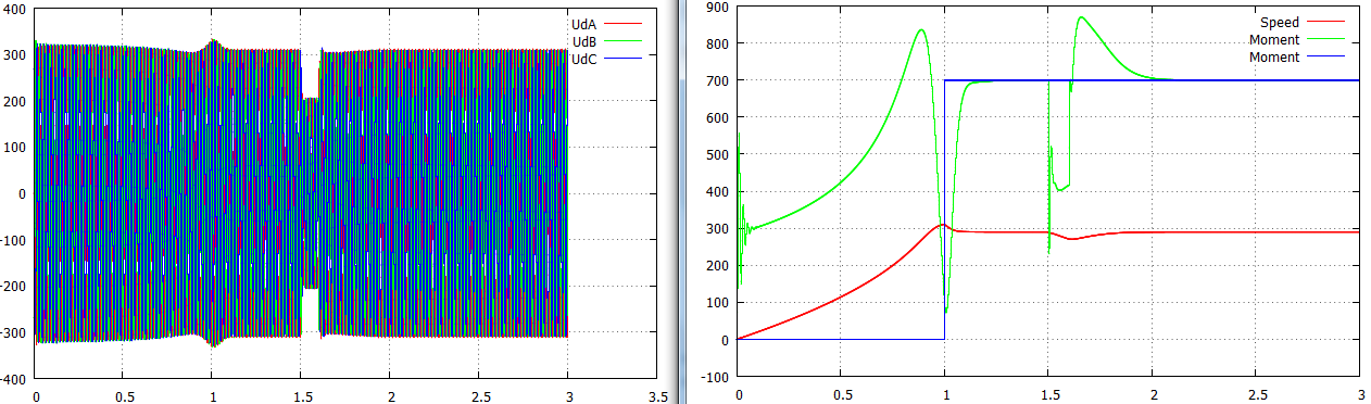
Figure 6 shows the process of starting an asynchronous motor. At time 1 s. A torque of 700 N * m is applied to the shaft and the engine goes into operating mode.
Fig. 6 - Graphs of the frequency of rotation of the motor shaft, as well as the torque on the shaft and the static torque when the engine is started
Parallel RLC - load -t rlc
This elementary node is a parallel connection of active resistance, inductance and capacitance. Depending on the parameters, it allows modeling the following standard and non-standard modes of exposure to a voltage source: one- and two-phase load, asymmetrical load, short circuit in phase short and long in time, short circuit to earth in all phases, short and long in time.
Table 5 - Configuration keys for the rlc node
| Key | Default value | Description |
| -Ra {ohm} -Rb {ohm} -Rc {ohm} | 0 (disabled) | Resistor in phase |
| -R {ohm} | 0 (disabled) | Resistance in all phases |
| -La {gn} -Lb {h} -Lc {gn} | 0 (disabled) | Inductance of the choke in phase |
| -L {H} | 0 (disabled) | Inductance of choke in all phases |
| -Ca {uF} -Cb {uF} -Cc {uF} | 0 (disabled) | Capacitor in phase |
| -C {μF} | 0 (disabled) | Capacitor capacitance in all phases |
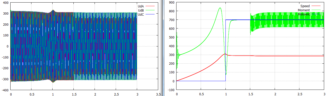
Simulate short-term short circuit in the network:
load -t acmotor -Rs 0.02 -Rr 0.02 -Ls 0.0008 -Lr 0.0002 -Lm 0.00015 -J 3 -p 2 -Ms 700 -Tload 1 load -t rlc -Ra 0.2 -Rb 0.2 -Rc 0.2 -On 1.5 -Off 1.6 KZ 0.1 s. The speed does not have time to fall below the critical, the engine restores speed after removing the short circuit.
load -t acmotor -Rs 0.02 -Rr 0.02 -Ls 0.0008 -Lr 0.0002 -Lm 0.00015 -J 3 -p 2 -Ms 700 -Tload 1 load -t rlc -Ra 0.2 -Rb 0.2 -Rc 0.2 -On 1.5 -Off 2 CZ 0.5 s, the engine has time to brake and after switching on the engine torque becomes less than the torque on the shaft and the engine crashes
load -t acmotor -Rs 0.02 -Rr 0.02 -Ls 0.0008 -Lr 0.0002 -Lm 0.00015 -J 3 -p 2 -Ms 700 -Tload 1 load -t rlc -Ra 0.2 -On 1.5 The closure in Phase A. The speed practically does not sag, because of the peculiarities of the asynchronous electric motor, it only needs two phases. The rotating magnetic field in the gap takes an oval shape and the shaft begins to vibrate with the frequency of the supply network.
Code optimization
In general, as it turned out, the main process of modeling itself was written quite accurately and no architectural changes were made according to the results of the modeling. But the devil is in the details.
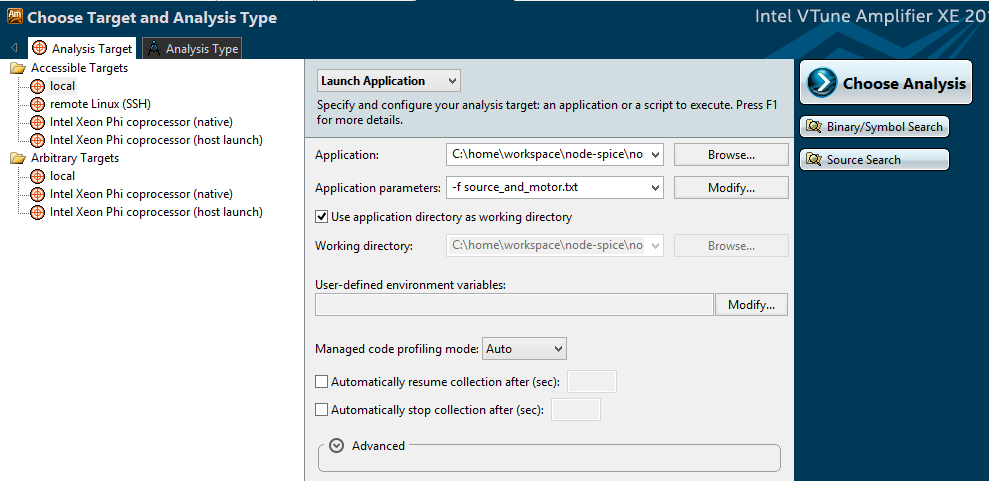
Open Intel Vtune Amplifier, create a new project:
Specify the path to our program and launch keys. It would be nice to use the Binary / Symbol Search and Source Search buttons and specify the paths to the source code and binaries with Debud-symbols - then it will be more convenient to navigate through the project and the source code.
We use the following config:
source_and_motor.txt one source, one motor
//create new solve system: setup -Off 10 -f 3200 //128 ticks per period load -t workbench -name wb0 load -t acsource -name ideal3f -f 50 -Ud 220 -R 0.1 //-L 0.001 load -t motor -name motor5 -On 0.5 -Off 4 -Rs 2 -Rr 0.8 -Ls 0.00991 -Lr 0.00991 -Lm 0.008419 -J 0.5 -p 2 -Ms 50 -Tload 2 -saveGraph//15kW load -t analyzer -name analyzer1 -tRMS 0.02 -U -I -P -E -Collect link -output ideal3f -input analyzer1 link -output analyzer1 -input motor5 solve graph All the above config files are in the / doc folder of the project.
Let's start with the simplest basic hotspot with an interval of 1ms
And run.
| Elapsed Time: | 52.548s |
| CPU Time: | 37.460s |
| Total Thread Count: | 1,035 |
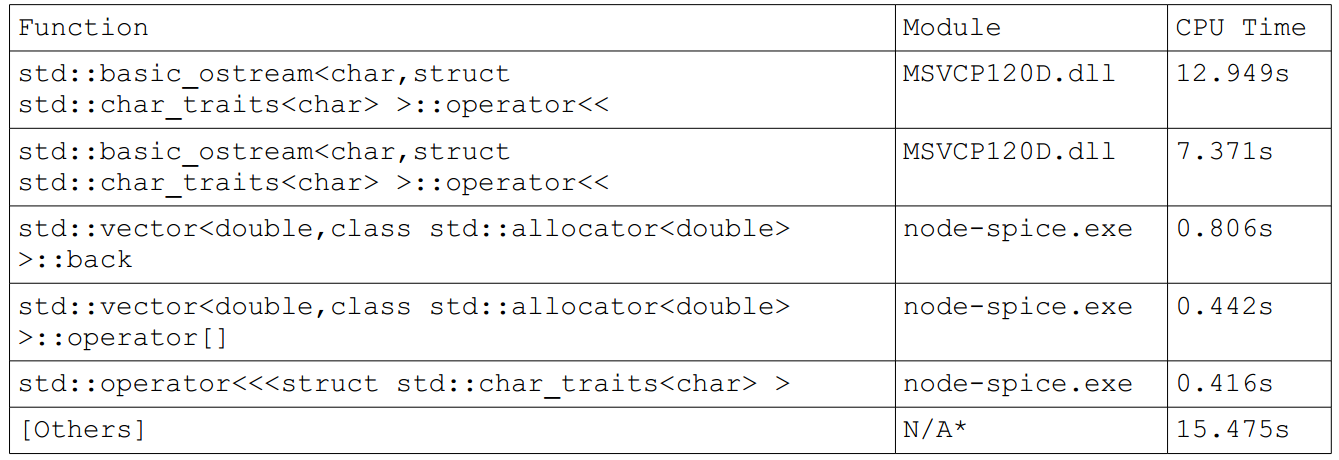
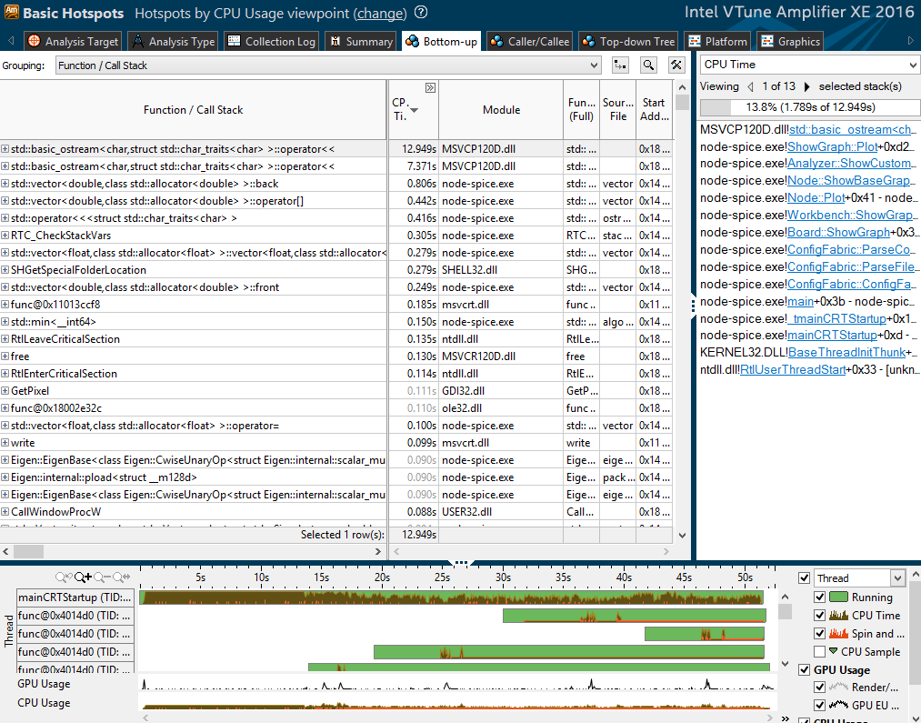
Top Hotspots:
Holy neutrons ... Of course, I knew that iostream is slow, but so much ... This, by the way, is disabling synchronization with
stdio ios_base::sync_with_stdio(false); 20 seconds of CPU time out of a total of 35 seconds. More than 50% of the time. It does not go into any gate.
You can read more about how slow the threads are here . It makes sense to rewrite everything to armored fprintf (). I was also interested that the cout function appears in the table twice. And for sure - the gnuplot layer creates temporary files and then deletes them. Add the -raw key to the node to save the raw graph files. There are keys - saved, no, not saved.
Run the profiler. Ha!
| Elapsed Time: | 22.421s |
| CPU Time: | 17.107s |
| Total Thread Count: | 1,035 |
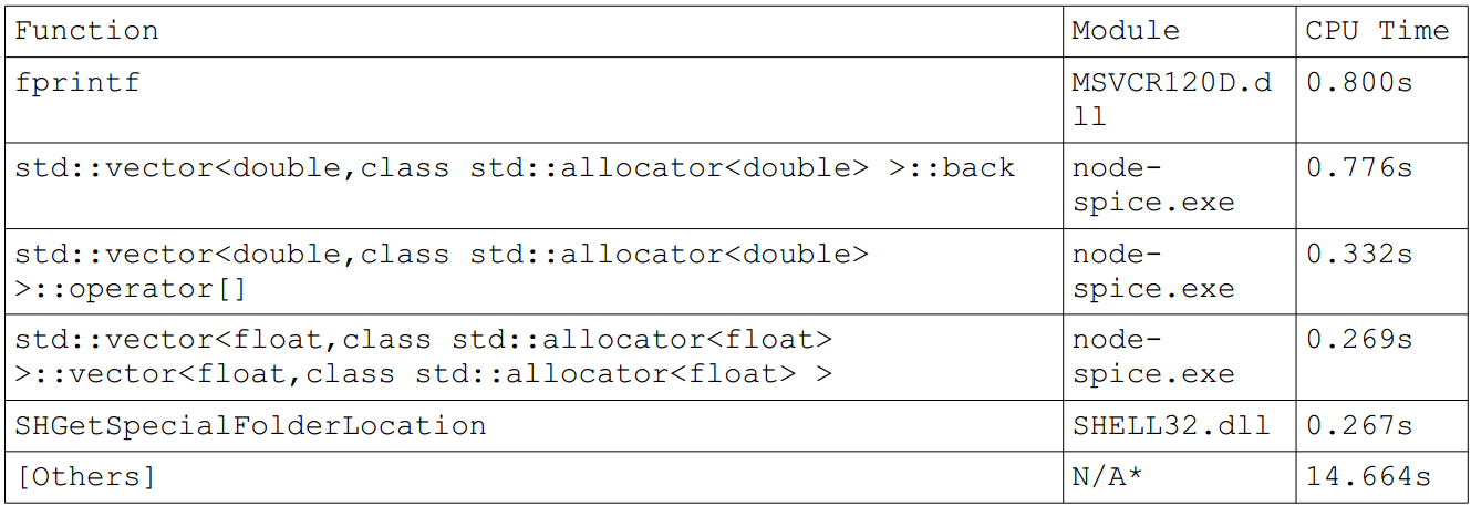
Top Hotspots:
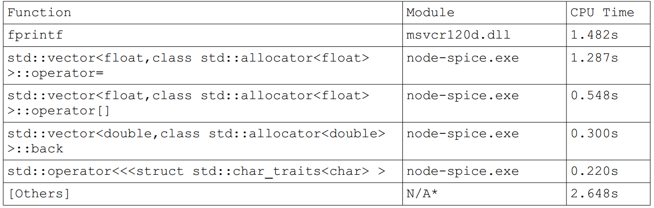
The leaders are still file output, but consuming less than 5% of CPU time. Serious success! Watch Bottom-Up three
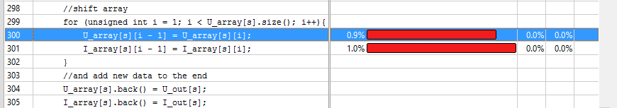
The second and third place is taken by pointers and iterators:
And that is quite logical - the place gets the power quality analyzer, because the latter does a lot of all the work.
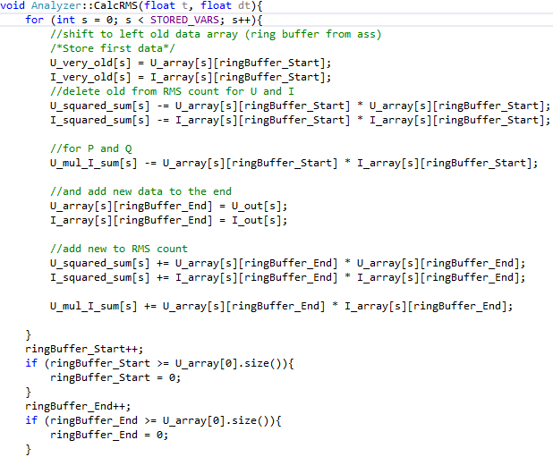
This code was written as a test of the concept of sliding measurement mode. As can be seen from the code, each new step of the solver is associated with a shift of a small (64-128 characters), but still an array. It makes sense to use a ring buffer to solve this problem. Then the operation of adding a new element will have the value O (1) instead of O (N).
“Why is this necessary?” You say, they say, the quality analyzer is one in the system, it is better to add motors to the config. And you will be half right - we will definitely add the motors, only analyzers in the system can be exactly as much as in the system of nodes - this is a feature of my thesis.
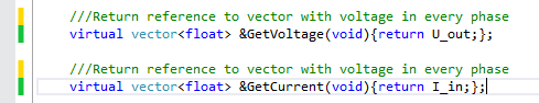
Let's look at what’s wrong with GetVoltage and GetCurrent bad:
Hmm, how about using links?
Restart profiling:
| Elapsed Time: | 23.197s |
| CPU Time: | 16.551s |
| Total Thread Count: | 1,048 |
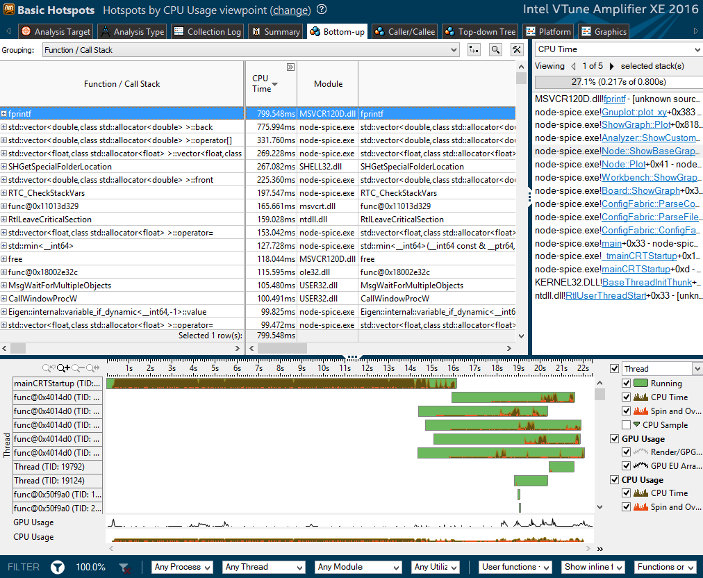
Top Hotspots:
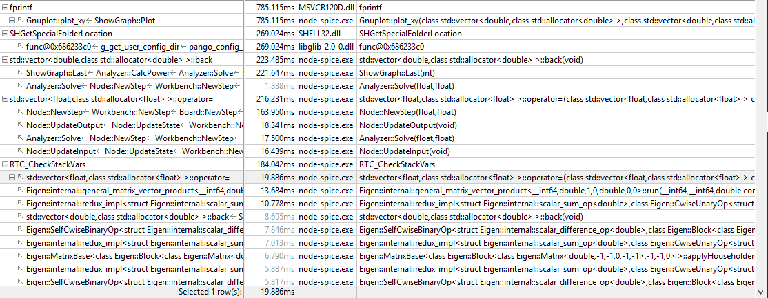
Bottom-Up three shows that, again, the first in the list is our fprintf and pango, crawling out from under the gnuplot - we’ll no longer be crawling into them (although it would be worth it).
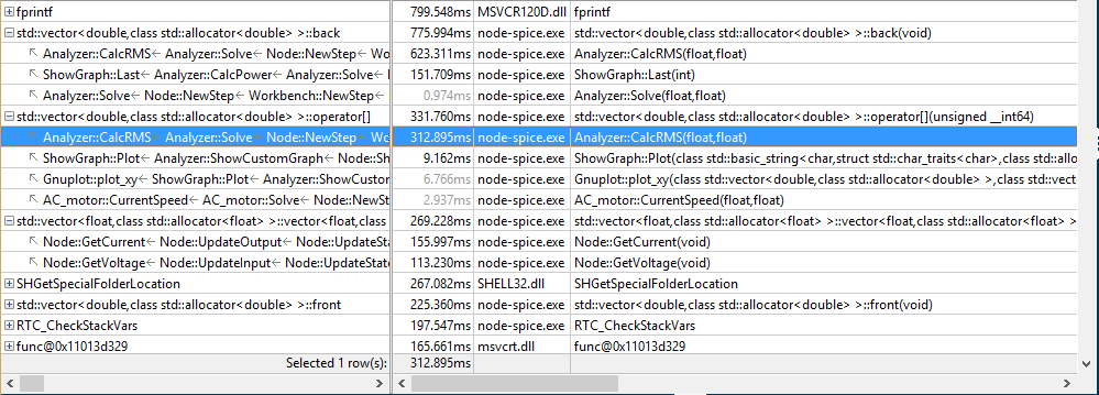
What really pleases is the fact that NewStep, from which a couple of steps to Solve took the lead. Run the simulation for 40 seconds and see how the picture changes:
| Elapsed Time: | 73.235s |
| CPU Time: | 61.790s |
| Total Thread Count: | 1,048 |
The effect is scaled, so here we have nothing to do.
Summarize
| It was | It became | Effect | |
| CPU Time: | 37.460s | 16.551s | 226% |
Not bad for half an hour of work?
Add to the engine heel system:
source_and_motors.txt: One source five motors
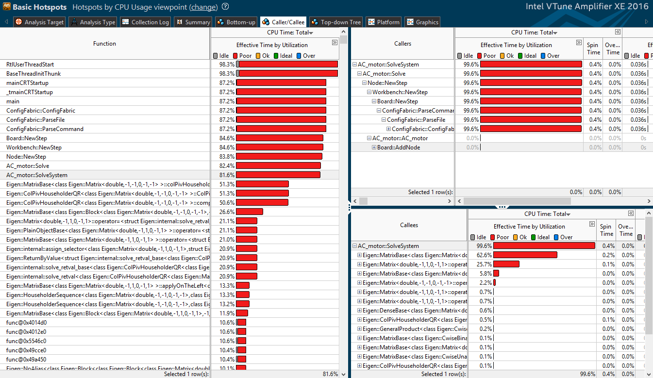
//create new solve system: setup -Off 10 -f 3200 //64 ticks per period load -t workbench -name wb0 load -t acsource -name ideal3f -f 50 -Ud 220 -R 0.1 //-L 0.001 load -t motor -name motor1 -On 0.5 -Off 5 -Rs 2 -Rr 0.8 -Ls 0.00991 -Lr 0.00991 -Lm 0.008419 -J 0.5 -p 2 -Ms 50 -Tload 2 -saveGraph//15kW load -t motor -name motor2 -On 1 -Off 6 -Rs 2 -Rr 0.8 -Ls 0.00991 -Lr 0.00991 -Lm 0.008419 -J 0.5 -p 2 -Ms 50 -Tload 2 -saveGraph//15kW load -t motor -name motor3 -On 1.5 -Off 7 -Rs 2 -Rr 0.8 -Ls 0.00991 -Lr 0.00991 -Lm 0.008419 -J 0.5 -p 2 -Ms 50 -Tload 2 -saveGraph//15kW load -t motor -name motor4 -On 2 -Off 8 -Rs 2 -Rr 0.8 -Ls 0.00991 -Lr 0.00991 -Lm 0.008419 -J 0.5 -p 2 -Ms 50 -Tload 2 -saveGraph//15kW load -t motor -name motor5 -On 2.5 -Off 9 -Rs 2 -Rr 0.8 -Ls 0.00991 -Lr 0.00991 -Lm 0.008419 -J 0.5 -p 2 -Ms 50 -Tload 2 -saveGraph//15kW load -t analyzer -name analyzer1 -tRMS 0.02 -U -I -P -E -Collect link -output ideal3f -input analyzer1 link -output analyzer1 -input motor1 link -output analyzer1 -input motor2 link -output analyzer1 -input motor3 link -output analyzer1 -input motor4 link -output analyzer1 -input motor5 solve graph From Bottom-Up three, little is clear:
Now, if you look at the Caller counter, you can see where the resources go. On the solution of matrix equations in the calculation of mat. motor models - most of the time the Eigen library is running.
We won’t get into the library; we’ll better replace the motors with rl-loads. They are much more important to me - you can create all sorts of different phase distortions, short circuits, disturbances and other joys.
Since we don’t really need to count anything on one tick, we’ll increase the clocking frequency of the solver, and we will increase the loads to 10 units.
source_and_rlc.txt One source and 10 RL loads
//create new solve system: setup -Off 10 -f 6400 //128 ticks per period load -t workbench -name wb0 load -t acsource -name ideal3f -f 50 -Ud 220 -R 0.1 //-L 0.001 load -t rlc -name rl1 -On 1 -Off 34 -Ra 100 -Rb 100 -Rc 100 -La 0.01 -Lb 0.01 -Lc 0.01 load -t rlc -name rl2 -On 2 -Off 35 -Ra 100 -Rb 100 -Rc 100 -La 0.01 -Lb 0.01 -Lc 0.01 load -t rlc -name rl3 -On 3 -Off 36 -Ra 100 -Rb 100 -Rc 100 -La 0.01 -Lb 0.01 -Lc 0.01 load -t rlc -name rl4 -On 4 -Off 37 -Ra 100 -Rb 100 -Rc 100 -La 0.01 -Lb 0.01 -Lc 0.01 load -t rlc -name rl5 -On 5 -Off 38 -Ra 100 -Rb 100 -Rc 100 -La 0.01 -Lb 0.01 -Lc 0.01 load -t rlc -name rl11 -On 11 -Off 24 -Ra 100 -Rb 100 -Rc 100 -La 0.01 -Lb 0.01 -Lc 0.01 load -t rlc -name rl21 -On 12 -Off 25 -Ra 100 -Rb 100 -Rc 100 -La 0.01 -Lb 0.01 -Lc 0.01 load -t rlc -name rl31 -On 13 -Off 26 -Ra 100 -Rb 100 -Rc 100 -La 0.01 -Lb 0.01 -Lc 0.01 load -t rlc -name rl41 -On 14 -Off 27 -Ra 100 -Rb 100 -Rc 100 -La 0.01 -Lb 0.01 -Lc 0.01 load -t rlc -name rl51 -On 15 -Off 28 -Ra 100 -Rb 100 -Rc 100 -La 0.01 -Lb 0.01 -Lc 0.01 load -t analyzer -name analyzer1 -tRMS 0.02 -U -I -P -E -Collect link -output ideal3f -input analyzer1 link -output analyzer1 -input rl1 link -output analyzer1 -input rl2 link -output analyzer1 -input rl3 link -output analyzer1 -input rl4 link -output analyzer1 -input rl5 link -output analyzer1 -input rl11 link -output analyzer1 -input rl21 link -output analyzer1 -input rl31 link -output analyzer1 -input rl41 link -output analyzer1 -input rl51 solve graph | Elapsed Time: | 11.008s |
| CPU Time: | 6.485s |
| Total Thread Count: | 1.245 |
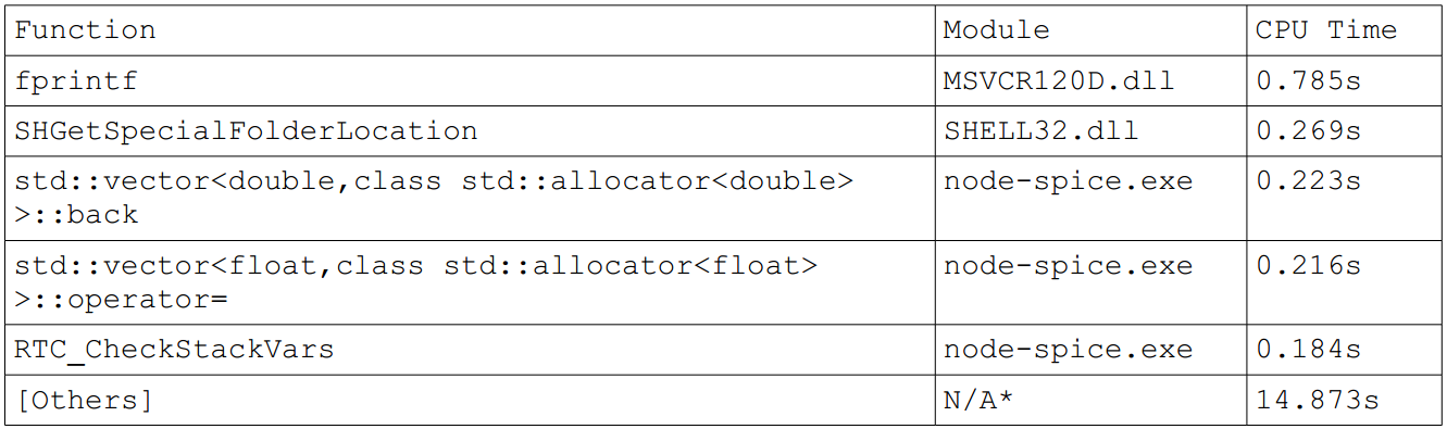
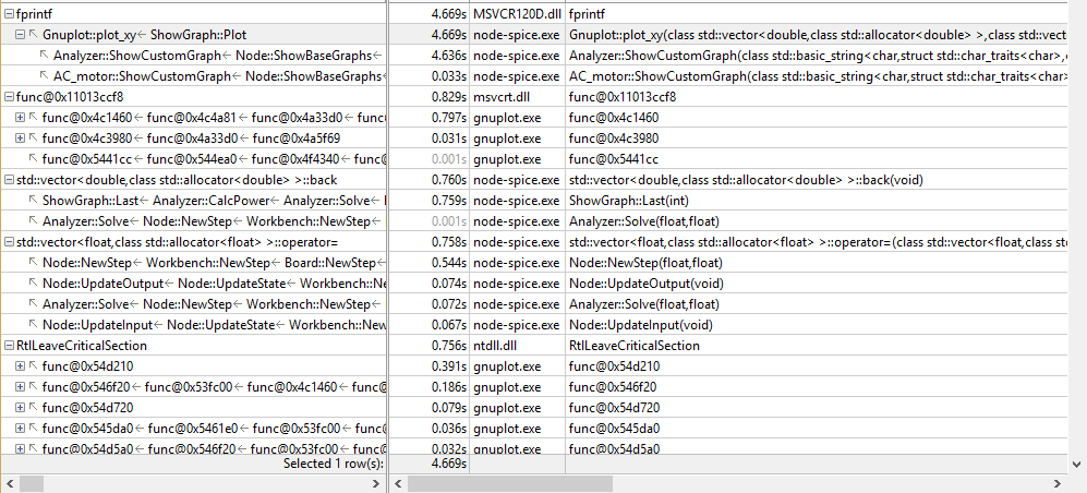
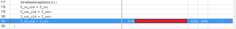
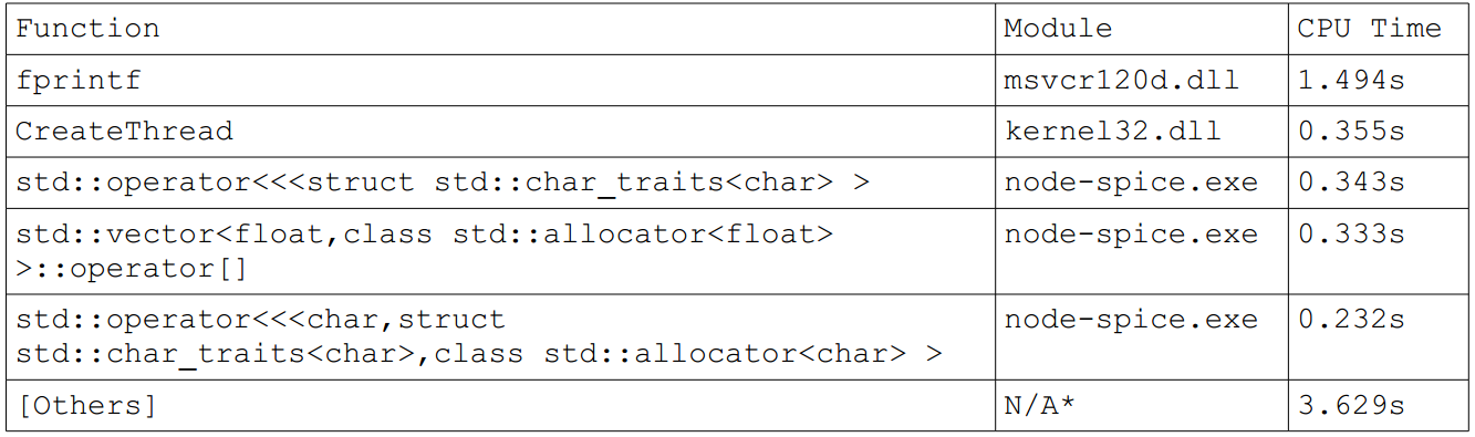
Fprintf we do not touch, but the main culprit:
Here we copy the double [4] vectors into each other. As you can see, vector copying by means of the vector itself is not very optimal. Zababahay we ka cycle - for 4 elements, especially it is not necessary to run out:
And the last time
| Elapsed Time: | 9.563s |
| CPU Time: | 6.386s |
| Total Thread Count: | 1.245 |
Findings:
And they do not have. I decided for myself that it was useless to upload brake applications in OpenSource and sat a little with a convenient and powerful profiling tool. In contrast to the placement of timestamps inside the code, Vtune, as they say, “pokes the muzzle” into a slow code, hinting that it would be nice to rewrite one or another piece.
My application, in fact, can be infinitely optimized - for a crutch on a crutch. You can throw out Eigen and rewrite Acmotor using Boost; you can write graph output on the same Boost; .
By the way, here you can get a free version of Intel parallel Studio for student and educational needs.
Source: https://habr.com/ru/post/301684/
All Articles