Structure from motion

If you look at the sequence of frames in which the camera moves, then the brain easily perceives the geometric structure of the content. However, in computer vision this is not a trivial problem. In this article I will try to describe a possible solution to this problem.

Before reading this article, it will not hurt to carefully read the article "Fundamentals of stereo vision" .

So, we are faced with the task of turning a sequence of two-dimensional images into a three-dimensional structure. The task is not simple, and you need to simplify it.
First, suppose that we only have two frames. Let's designate them as A and B.
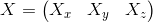
Secondly, we will work with a finite set of points corresponding to each other on frames A and B. Denote the points on the image as . Then the points on frames A and B will be and . Each pair of points corresponds to a point in three-dimensional space. .

Now you need to decide how to search. and . To do this, on the first frame we will select points, with the greatest contrast - “special” points (features). For this you can use surf, fast or something else . These points will be . Then it is necessary to find correspondences to these points on the second frame using the same surf or optical flow algorithm. And this is the point .
')
And now we come to the central question of this article: how from the points and (point-correspondences, point correspondences) get the coordinates of the points and the position of the camera in space? First you need to figure out how the point it falls on the image. Need to build a mathematical model of the camera.

Projective Camera Model

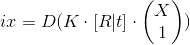
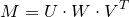
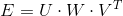
Since you have probably already read the article "Fundamentals of stereo vision", this formula should be familiar:
.
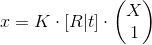Or if you describe more fully:
.
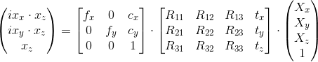Here X is a three-dimensional point in space.
x is the coordinate of the point in the image in uniform coordinates , and 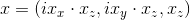i.e. the translation to the usual coordinates of the image will be as follows: .
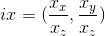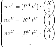
The process of converting a point in space to image coordinates can be divided into two stages, implemented by two matrices in the formula:

1. [R | t] - R and t represent the position of the camera in space. At this stage, the coordinates of the points are transferred to the local coordinates of the camera. R is a 3x3 rotation matrix, t is a three-dimensional displacement vector - together they make up the transition matrix [R | t] (3x4 size), it determines the position of the camera in the frame. [R | t] is the same as the view matrix in three-dimensional graphics (if you do not take into account that it is not 4x4 in size).
   - this is a matrix of camera rotation, - three-dimensional coordinates of the location of the camera in space. R and t are called external camera parameters.
2. K is the matrix of the camera. The local coordinates of the points are converted to homogeneous coordinates of the image. f _x , f _y - the focal distance in pixels, c _x , c _y - the optical center of the camera (usually the coordinates of the center of the image). These parameters are called internal camera parameters.

An important property of this model is that the points lying on one straight line in space will also lie on one straight line on the image.
In fact, the described model can be very inaccurate. In real cameras, lens distortions come into play, due to which straight lines become curves. This distortion is called distortion . There are different models that correct these distortions. Here are some of their implementations. The parameters of this model are also included in the concept of internal camera parameters.
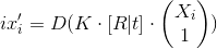
Given the distortion of our formula is complicated:
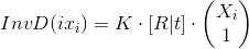
, where D (X) is a function that takes homogeneous coordinates of image points and returns normal coordinates on the image. We also need the inverse function later, InvD (ix).
Internal camera parameters must be known in advance. Clarification of these parameters is a separate topic, we will assume that they already exist.

Distortion distortion does not depend on the depth of visible points, but only the coordinates in the image. It means that you can “fix” the image (getting straight lines where they should be) without knowing the external parameters of the camera and the coordinates of points in space. Then you can use the camera model without the function D.

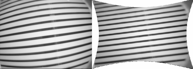
The image with distortion on the left and on the right is the “corrected” image from lens distortions. It is seen that the lines were straight.

Normalization of points

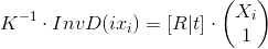
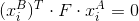
We agreed that the internal parameters are known to us, the coordinates of points on the image are known, and therefore it remains to find [R | t] and X _i (camera positions and points in space).
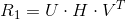
Our formula is already a little complicated, we need to simplify it. To begin, do this:

The expression remains fair. We continue:

Denote 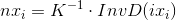(and if without distortion, then 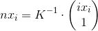). Since all parameters are known, nx _i can be calculated in advance. Recalling how the matrix K looks like, it can be understood that nx _z = 1. This will help with further calculations. As a result, the formula becomes simpler:


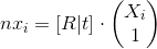
nx _i are the normalized points of the image.

Fundamental and Essential Matrices

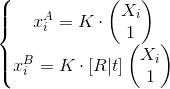
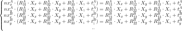
So, suppose we have two images taken from the same camera. We do not know the position of the cameras and the coordinates of points in space. We agree to enter calculations regarding the first frame. So it turns out that RA = I (I is the identity matrix), t ^A = (0, 0, 0). The camera position in frame B is simply denoted as R and t (i.e., R ^B = R, t ^B = t). [R | t] is the matrix of the coordinates of the second frame, and it is also the matrix of the displacement of the camera position from frame A to frame B. As a result, we get such a system (disregarding distortion!):

Using the fundamental matrix F (fubdamental matrix), we obtain the following equation:

Also note that F has a size of 3x3 and must have a rank equal to 2.
From the fundamental matrix F it is already possible to obtain the necessary R and t. However, distortion spoils everything, with its account the dependence of points between frames will be non-linear, and this will no longer work.
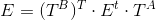
But we proceed to the normalized points and use the essential matrix E (essential matrix). Everything will be almost the same, but simpler:
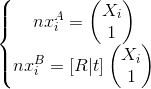- The system of equations for the essential matrix;
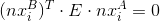- the equation for her.
And here we can safely take into account distortion.
The fundamental and essence matrices are connected in this way:

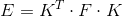
Now we are faced with the task of finding either the fundamental matrix F, or the essence matrix E, from which we can later get on R and t.

Essence matrix calculation (8-point algorithm)

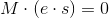
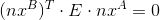
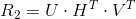
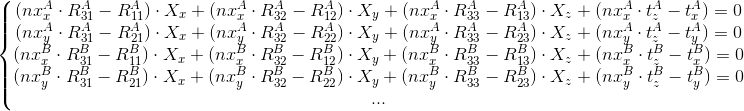
Let's return to the equation:

The same formula can be rewritten in this form (we recall that and ):
, the parameter i is omitted here for the sake of convenience, but we mean that this is true for each point.
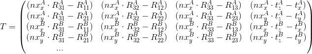
We introduce the vector e and the matrix M:


Then the whole system of equations can be represented as:

We obtain a homogeneous system of equations, having solved which, we obtain E from e. The zero vector is the obvious solution, but we are clearly not interested in it. At least 8 points are required for solving.

Solving systems of homogeneous equations using singular expansion

The singular decomposition is a decomposition of the matrix, leading it to this form:
where U, V are orthogonal matrices, W is a diagonal matrix. In this case, the diagonal elements of the matrix W are usually arranged in descending order. Also the rank of the matrix W is the rank of the matrix M. And since W is a diagonal matrix, its rank is the number of nonzero diagonal elements.

So, the following equation was given:
, where M is the known matrix, e is the vector that is not necessary to find.

The rows V ^T , to which the zero diagonal element W on the same line corresponds, are the null-spaces of the matrix M, that is, in this case, are linearly independent solutions of our system. And since the elements of W are arranged in descending order, then you need to look at the last element of the matrix W. And the solution will be the last line .
When calculating an entity matrix using 8 points, the last element of the matrix W should be zero - W ₉₉ = 0, but in practice, due to errors, there will be some non-zero value, and the magnitude of this value can be used to estimate the magnitude of this error. In this case, we get the best solution.
Nevertheless, the solution we found is not the only one; moreover, there will be infinitely many solutions. If you multiply the solution found by a factor, it will still remain a solution. Thus, the coefficient hid in the equation (which can be any):
.
True, all these decisions will be linearly dependent, and only one of them will be of interest to us.
Hence the matrix E can also be scaled. But the calculations are carried out in a homogeneous space and, as a result, they do not depend on the scaling (i.e., on the coefficient s).
It is probably worth scaling the resulting matrix E so that E ₃₃ = 1.

Calculation of an essence matrix (7-point algorithm)

You can do with 7 points.
If we take only 7 points, then M will be a 7x9 matrix.
Let's return to the expression:

W - will also be a 9x9 matrix, as before, but now not only W ₉₉ will be equal to zero (well, again without taking into account calculation errors), but also W ₈₈ . This means that we have two linearly independent solutions of the equation . From them we obtain two matrices E ₁ and E ₂ . The solution will be the expression .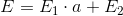
Essential matrix, as well as the fundamental, must have a rank equal to two, and since it has a size of 3x3, then the determinant of the matrix is ​​0 - . Consequently 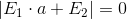. If we paint this equation, we get a cubic equation that has 1 or 3 solutions . So we get one or three matrix E.
I will not paint the solution of this equation (it is voluminous, well, consider this as homework). In a pinch, you can just watch the implementation in opencv right away.

Refinement of the essential (fundamental) matrix

Since everything in this world is imperfect, we will constantly receive mistakes that we need to fight. So the essential matrix must have a rank equal to 2 and therefore . In practice, however, this will not be the case.
To see what this is expressed in, let's take the fundamental matrix. Essential matrix / fundamental matrix - the only difference is in what points we work with (normalized or points on the image).
A ray emitted from point A of frame A will fall into frame B as a straight line (or not entirely due to distortion, but forget about it). Suppose matrix F is the fundamental matrix of frames A and B ( ).
Then if you release the beam from the point , then we get a straight line l on the frame B - . This straight line is called the epipolar line, i.e. where ix, iy are the coordinates of a point in the image. And the same condition for a point on an image with homogeneous coordinates - . Point will lie on this line, therefore . Hence comes the general formula - .

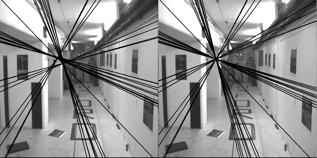
The picture shows an example of the epipolar lines obtained from the correct fundamental matrix (the rank of which is 2, the picture on the right) and the wrong one (on the left).
To get the correct fundamental matrix, we use the singularity decomposition property — to bring the matrix closer to a given rank:
. Ideally, W ₃₃ (the last element of the diagonal) should be zero. We introduce a new matrix W ', which is equal to W, only in which the element W' ₃₃ = 0.
Then the corrected version: .
Exactly the same principle works for the essential matrix.

Normalized version of the algorithm

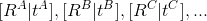
To reduce the error obtained in the calculations, the points transform to a specific view. Matrices T ^A and T ^B are selected, which (each independently and on its own frame) shift the average coordinate of the points to the point (0, 0) and scale so that the average distance to the center is equal to :

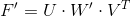
A matrix T ^{A, B} have the form: , where c is the average coordinate of the frame points, s is the scale factor.
After that, we calculate the entity matrix as usual. After it is necessary to clarify it, as described above. Denote the resulting matrix as E ^t .
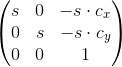
Summary Entity Matrix - .
Eventually:
Again, if you need to find a fundamental matrix, all principles are preserved.

Getting the camera position from the entity matrix

We introduce the matrix H:
We use singular decomposition on the essential matrix:
Then we get the following solutions:



where , - coordinates of the camera position.
We also need the position of the camera in the local coordinates of the camera itself: .
There are four solutions: .
In the case of an 8-point algorithm, choose from 4 solutions. In the case of the 7-point algorithm, there will be three essence matrices, from which 12 solutions will be obtained. You need to choose only one, the one that will give less errors.

Degenerate cases

Let us return to the calculation of the essence matrix. We had the equation:

Then we solved it with the help of singular decomposition:

Solutions of this equation depend on the rank of the matrix W, well, or on the number of zeros in the diagonal of this matrix (we remember that this reflects the rank of the matrix). That's just taking into account the error, we consider zero in this case a number that is close enough to zero.
We have such options:

• No zeros. No solutions, probably the error came out too big.
• One zero. One solution, the case in which the number of points is greater than or equal to eight.
• Two zeros. One or three solutions. Used seven or more points.
• Three zeros. Then the condition should be true . This is possible if the camera did not move from frame to frame, there was only a turn, that is, t = (0, 0, 0). Or all points lie on the same plane. In the second case, it is still possible to find the coordinates of these points and the position of the camera, but in other ways.

Calculation of coordinates of points in space

Suppose now we have more than two frames - A, B, C, ...
- the position of the camera frames A, B, C, ...
- normalized points
Need to find the point

Imagine this system as:


In matrix form:


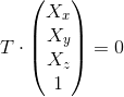
Using singular decomposition we find the vector , which the (as described above). Then 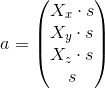where s is some unknown coefficient. Coming out .

Evaluation function

Cost functions are necessary in order to obtain some results, to assess how reliable they are, or to compare them with others.
Take our model:
- the intended result.
- the real value of the point.
Hence, the square of the error for the i-th point will be: .
In practice, some points will give more reliable results than others. And some in general will obviously give the wrong ones. As a result, it becomes necessary to select from the general array of points only those points that can be trusted, and the rest simply be discarded from the calculations.
The easiest way to select “reliable” points is to select a certain limit (say, 5 pixels), and take only those points that give an error less than this limit ( ). It should also be noted that it is necessary to take into account that the point must lie in front of the camera in both frames, otherwise it must clearly be discarded.
Thus, you can enter the evaluation function - the number of reliable points. And when comparing, choose the result that gives a greater number of “reliable” points.
And you can use another, more “thin” function:
where limit is our chosen limit (5 pixels).
The best option is the one that will give less value. It is clear that here you should remove the “unreliable” points for future calculations.

RANSAC method

1. When calculating the essence matrix, it is necessary to discard “unreliable” points, as they result in significant errors in the calculations. You can determine the set of suitable points using the RANSAC algorithm.
   Repeat the cycle a specified number of times (for example, 100, 400):
   
   • We randomly select the minimum set of points for calculations (we have 7);
   • We calculate the essence matrices from this set (I recall, it can turn out to be either one matrix or three)
   • The evaluation function calculates the reliability of each matrix
2. From the previous cycle, we select the essence matrix, which gives the best result;
3. We choose points for calculations that give an error when the error matrix obtained is an error less than the specified threshold;
4. From the obtained set of points, we calculate the final essence matrix.

General algorithm

1. Find the “special” points on the first frame.
2. We define the point of correspondence between the two images.
3. We find the essential (or, nevertheless, fundamental) matrix corresponding to these two images using RANSAC.
4. We will have one or three solutions, from which we obtain 4 or 12 possible matrices [R | t]. Having the position of the cameras in both frames, we calculate the coordinates of points in space for each possible matrix. From them we choose the best one using the evaluation function.

What's next?

Initially, we proceeded from the assumption that we had only two frames.
To work with a sequence of frames, you just need to split the sequence into successive pairs of frames. By processing pairs of frames, we get the shift of the camera from one frame to another. From this you can get the position coordinates of the camera in the remaining frames.

Having received the main thing - the position of the cameras, you can act in different ways:

• By the points-correspondences to get the three-dimensional coordinates of the points in space, a cloud of points will be released, which can be turned into a three-dimensional model.
• Use the fundamental matrix to calculate the depth map.
• Using two frames to initialize the map for SLAM using the calculated coordinates of points in space, it is possible to quickly and easily obtain the position coordinates in the following frames.
• well and another

In general, you can act differently, using different methods, including those algorithms that have been described - are not the only ones.

Literature

Fundamental matrix , Essential matrix , Eight-point algorithm - more information on Wikipedia
Hartley, Zisserman - Multiple View Geometry in Computer Vision - sponsored by this article