Hopfield neural network on fingers

The article is devoted to the introduction of neural networks and the example of their implementation. The first part gives a small theoretical introduction to neural networks on the example of the Hopfield neural network. It is shown how the network is trained and how its dynamics are described. The second part shows how to implement the algorithms described in the first part using the C ++ language. The developed program clearly shows the ability of the neural network to clear the key image from noise. At the end of the article there is a link to the source code of the project.

Theoretical description

Introduction

To begin with, it is necessary to determine what a neuron is. In biology, a neuron is a specialized cell that makes up the nervous system. Biological neuron has the structure shown in Fig.1.

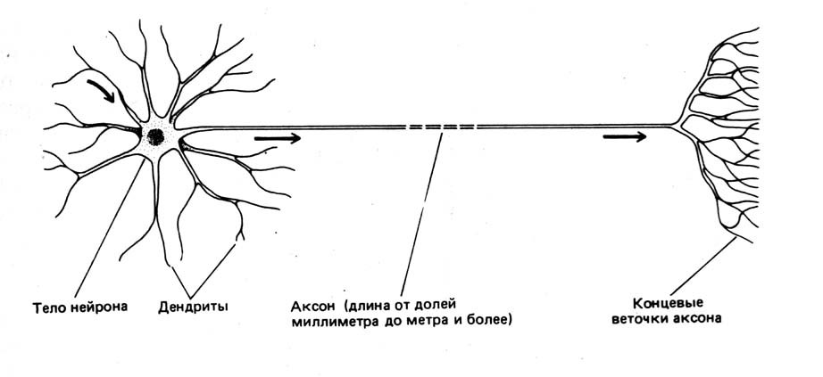
Fig.1 Scheme of the neuron

A neural network can be entered as a collection of neurons and their interconnections. Therefore, in order to define an artificial (non-biological) neural network, it is necessary:

Set the network architecture;
Determine the dynamics of individual elements of the network - neurons;
Determine the rules by which neurons interact with each other;
Describe the learning algorithm, i.e. formation of relationships to solve the problem.

The Hopfield network will be used as the neural network architecture. This model seems to be the most common mathematical model in neuroscience. This is due to its simplicity and clarity. The Hopfield network shows how memory can be organized in a network of elements that are not very reliable. Experimental data show that with an increase in the number of failed neurons to 50%, the probability of a correct answer is extremely close to 100%. Even a superficial comparison of the neural network (for example, the brain) and the Von Neumann computer shows how strongly these objects differ: for example, the frequency of changes in the states of neurons ("clock frequency") does not exceed 200 Hz, while the frequency of changes in the state of the elements of a modern processor can reach several GHz ( $10 ^ 9$ Hz).
Formal description of the Hopfield network

The network consists of N artificial neurons, the axon of each neuron is associated with the dendrites of the rest of the neurons, forming a feedback. The network architecture is shown in Fig. 2

Fig.2 Hopfield neural network architecture

Each neuron can be in one of 2 states:

$S (t) \ in \ {- 1; +1 \}$

Where $S (t)$ - the state of the neuron at the time $t$ . "Excitement" of the neuron corresponds $+1$ , and "braking" $-one$ . The discreteness of the states of the neuron reflects the non-linear, threshold nature of its functioning and is known in neurophysiology as the “all or nothing” principle.

State dynamics over time $i$ -th neuron in the network from $N$ neurons are described by a discrete dynamic system:

$S_ {i} (t + 1) = sign [\ sum \ limits_ {j = 1} ^ N J_ {i, j} S_ {i} (t)], \ quad i, j \ in1, .., N$

Where $J_ {i, j}$ - matrix of weight coefficients describing the interaction of dendrites $i$ 2nd neuron with axons $j$ th neuron.

It is worth noting that $J_ {i, i} = 0, \ quad i = 1, .., N$ and case $\ sum \ limits_ {j = 1} ^ {N} J_ {i, j} S_ {i} (t) = 0$ not considered.

Training and noise resistance

Hopfield network training for weekend images $\ zeta _ {\ mu} ^ {in}$ reduced to calculating the values of matrix elements $J_ {i, j}$ . Formally, we can describe the learning process in the following way: let it be necessary to train the neural network to recognize $M$ images marked $\ {\ zeta _ {\ mu} ^ {in}, \ mu = 1, .., M \}$ . Input image $\ overline {\ zeta _ {\ mu} ^ {in}}$ represents: $\ overline {\ zeta _ {\ mu} ^ {in}} = \ zeta _ {\ mu} ^ {in} + \ acute {\ zeta}$ Where $\ acute {\ zeta}$ - noise superimposed on the original image $\ zeta _ {\ mu} ^ {in}$ .
In fact, neural network training is the definition of the norm in the image space. $|| \ zeta _ {\ mu} ^ {in} - \ overline {\ zeta _ {\ mu} ^ {in}} ||$ . Then, clearing the input image from noise can be described as minimizing this expression.

An important characteristic of the neural network is the ratio of the number of key images $M$ that can be memorized, to the number of neurons in the network $N$ : $\ alpha = \ frac {M} {N}$ . For the Hopfield network value $\ alpha$ not more than 0.14.

Calculation of a square matrix of size for key images is made according to Hebb's rule:

$J_ {i, j} = {1 \ over N} \ cdot \ sum \ limits _ {\ mu = 1} ^ {M} \ big [\ zeta_ {i, \ mu} ^ {in} \ cdot \ zeta_ {j , \ mu} ^ {in} \ big]}$

Where $\ zeta_ {j, \ mu} ^ {in}$ means $j$ element of the image $\ zeta _ {\ mu} ^ {in}$ .

It should be noted that due to the commutativity of the multiplication operation, the equality
$J_ {i, j} = J_ {j, i}$

The input image that is presented for recognition corresponds to the initial data for the system, which serves as the initial condition for the dynamic system (2):

$S_ {i} = \ overline {\ zeta _ {\ mu} ^ {in}}$

Equations (1), (2), (3), (4) are sufficient to determine the Hopfield artificial neural network and you can proceed to its implementation.

Hopfield neural network implementation

The implementation of the Hopfield neural network defined above will be done in C ++. To simplify the experiments, we add the basic definitions of types that are directly related to the type of neuron and its transfer function in the class simple_neuron , and we define derivatives later.

The most basic types directly associated with a neuron are:

type of weight coefficients ( float selected);
A type that describes the state of the neuron (an enumerated type is entered with 2 valid values).

Based on these types, you can enter the remaining basic types:

The type that describes the state of the network at the time $t$ (standard vector container is selected);
A type describing the matrix of weights of neuron connections (the vector container vector is selected).

Listing 1. Defining new types

struct simple_neuron { enum state {LOWER_STATE=-1, UPPER_STATE=1}; typedef float coeff_t; <<(1) typedef state state_t; <<(2) ... }; typedef simple_neuron neuron_t; typedef neuron_t::state_t state_t; typedef vector<state_t> neurons_line; <<(3) typedef vector<vector<neuron_t::coeff_t>> link_coeffs; <<(4)

Network training, or, calculation of matrix elements $J_ {i, j} = J_ {j, i}$ In accordance with (3), it is produced by the learn_neuro_net function, which accepts a list of training images as input and returns an object of the type link_coeffs_t . Meanings $J_ {i, j}$ calculated for lower triangular elements only. The values of the upper triangular elements are calculated in accordance with (4). A general view of the learn_neuro_net method is shown in Listing 2.

Listing 2. Neural network training

 link_coeffs learn_neuro_net(const list<neurons_line> &src_images) { link_coeffs result_coeffs; size_t neurons_count = src_images.front().size(); result_coeffs.resize(neurons_count); for (size_t i = 0; i < neurons_count; ++i) { result_coeffs[i].resize(neurons_count, 0); } for (size_t i = 0; i < neurons_count; ++i) { for (size_t j = 0; j < i; ++j) { neuron_t::coeff_t val = 0; val = std::accumulate( begin(src_images), end(src_images), neuron_t::coeff_t(0.0), [i, j] (neuron_t::coeff_t old_val, const neurons_line &image) -> neuron_t::coeff_t{ return old_val + (image[i] * image[j]); }); result_coeffs[i][j] = val; result_coeffs[j][i] = val; } } return result_coeffs; }

Neuron states are updated using the neuro_net_system functor. The argument of the _do functor method is the initial state $S_ {i} (0)$ , which is a recognizable image (in accordance with (5)) - a reference to an object of type neurons_line .

The functor method modifies the transmitted object of type neurons_line to the state of the neural network at the moment of time $T$ . The value is not fixed and is determined by the expression:

$S_ {i} (T-1) = S_ {i} (T)$

i.e., when the state of each neuron has not changed in 1 “cycle”.

To calculate (2), 2 STL algorithms are applied:

std :: inner_product to calculate the sum of the products of weights and neuron states (i.e., calculation (2) for a specific $i$ );
std :: transform to calculate new values for each neuron (i.e., calculate the item above for each possible $i$ )

The source code for the neurons_net_system functor and the calculate method for the simple_neuron class is shown in Listing 3.

Listing 3. A functor that implements a neural network

 struct simple_neuron { ... template <typename _Iv, typename _Ic> static state_t calculate(_Iv val_b, _Iv val_e, _Ic coeff_b) { auto value = std::inner_product( val_b, val_e, coeff_b, coeff_t(0) ); return value > 0 ? UPPER_STATE : LOWER_STATE; } }; struct neuro_net_system { const link_coeffs &_coeffs; neuro_net_system(const link_coeffs &coeffs): _coeffs(coeffs) {} bool do_step(neurons_line& line) { bool value_changed = false; neurons_line old_values(begin(line), end(line)); link_coeffs::const_iterator it_coeffs = begin(_coeffs); std::transform( begin(line), end(line), begin(line), [&old_values, &it_coeffs, &value_changed] (state_t old_value) -> state_t { auto new_value = neuron_t::calculate( begin(old_values), end(old_values), begin(*it_coeffs++) ); value_changed = (new_value != old_value) || value_changed; return new_value; }); return value_changed; } size_t _do(neurons_line& line) { bool need_continue = true; size_t steps_done = 0; while (need_continue) { need_continue = do_step(line); ++steps_done; } return steps_done; } };

To output input and output images to the console , a neurons_line_print_descriptor type has been created that stores a link to the image and the formatting format (the width and height of the rectangle in which the image will be written). For this type, the operator << is overridden. The source code for the neurons_line_print_descriptor type and the output operator is shown in Listing 4.

Listing 4. Outputting the state of a neural network to a stream

 struct neurons_line_print_descriptor { const neurons_line &_line; const size_t _width; const size_t _height; neurons_line_print_descriptor ( const neurons_line &line, size_t width, size_t height ): _line(line), _width(width), _height(height) {} }; template <typename Ch, typename Tr> std::basic_ostream<Ch, Tr>& operator << (std::basic_ostream<Ch, Tr>&stm, const neurons_line_print_descriptor &line) { neurons_line::const_iterator it = begin(line._line), it_end = end(line._line); for (size_t i = 0; i < line._height; ++i) { for (size_t j = 0; j < line._width; ++j) { stm << neuron_t::write(*it); ++it; } stm << endl; } return stm; }

Neural network operation example

To test the performance of the implementation, the neural network was trained in 2 key images:

Fig.3 Key images

At the entrance were distorted images. The neural network correctly recognized the original images. Distorted images and recognized images are shown in Fig.4, 5

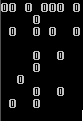
Fig.4. Pattern Recognition 1

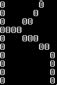
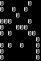
Fig.5 Pattern Recognition 2

The program is launched from the command line with the following line: AppName WIDTH HEIGHT SOURCE_FILE [LEARNE_FILE_N], where:

  AppNaame - the name of the executable file;
 WIDTH, HEIGHT - the width and height of the rectangle into which the output and key images will fit;
 SOURCE_FILE - source file with the initial image;
 [LEARNE_FILE_N] - one or more files with key images (separated by spaces).

The source code is posted on GitHub -> https://github.com/RainM/hopfield_neuro_net

The CMake project is in the repository, from which you can generate a Visual Studio project (VS2015 compiles the project successfully) or regular Unix Makefiles.

References

G.G. Malinetsky Mathematical foundations of synergy. Moscow, URSS, 2009.
The article "Neuronnetwork_Hopfilda" on Wikipedia.

Source: https://habr.com/ru/post/301406/

All Articles