Preamble

I continue the detailed description of the use of a linear-quadratic regulator on the example of control of an inverted pendulum. By the way, the term “LCR” very inaccurately captures the essence of what is happening, as I have already been suggested in the comments, in the Russian school of control theory this approach is called “analytical design of optimal regulators”, which is significantly more accurate.

As usual, I try to chew up the math to the maximum so that the material is available to the interested student. I am deeply convinced that the use of mathematics in an amicable way should be paid: any formula should be used only when it is intended to facilitate understanding, and not to show off.

So, this is the fourth article, for a better understanding of what is happening, it would be nice to read the previous three:

• 1. Least squares methods
• 2. Linear square controller, introductory
• 3. DC motor control with linear-square controller

')
Here is a picture of the system (clickable):

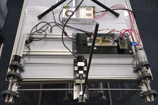
Used sensors

I have only two sources of information about what is happening in the system, these are two incremental encoders, one (1000 pulses per revolution) indicates the position of the carriage, the second (2000 pulses per revolution) gives the position of the pendulum itself. In the previous article I considered pulses with the help of the Arduin itself, but this is rather inaccurate and poorly resistant to noisy readings of encoders. In addition, it spends the already weak computing resources atmega. Now I have installed one HCTL-2032 microcircuit (about five euros per aliexpress), it can count the pulses of two encoders, providing 32-bit counters for this. To save Arduin's legs, there is 74hc165 between the counter and the Arduina itself, reading one byte in parallel and delivering this byte in series.

We measure the parameters of the engine again

Compared to the previous article, I have slightly changed the system parameters (another engine driver plus put the encoder on the carriage), so I measure the system parameters again. So, with a small step (about one volt, from -24V to 24V), I apply a constant voltage to the motor and measure the change in the speed of the carriage. The carriage speed is considered as the difference between the adjacent carriage positions divided by the past tense (the correctness of this approach is later). The code used can be seen here .

Horizontal time in seconds, and the vertical speed of the carriage in meters per second. Noisy curves are the results of a real measurement; smooth curves are my mathematical model of the system. At present, the task is to calculate the model for smooth curves that approximate reality.



It turned out that I had slightly overdone it with a motor, at 24V the carriage accelerates by about 60 meters per second per second and the system's rigidity is not enough for a reasonable measurement of anything. Therefore, I cut the measurements at fifteen volts; in the initial part of the curves one can see oscillations in the speed of the carriage.

So, for each measurement, I consider the steady-state speed (plateau height) and draw a graph, on which the applied voltage is horizontally and the steady-state speed is vertical.



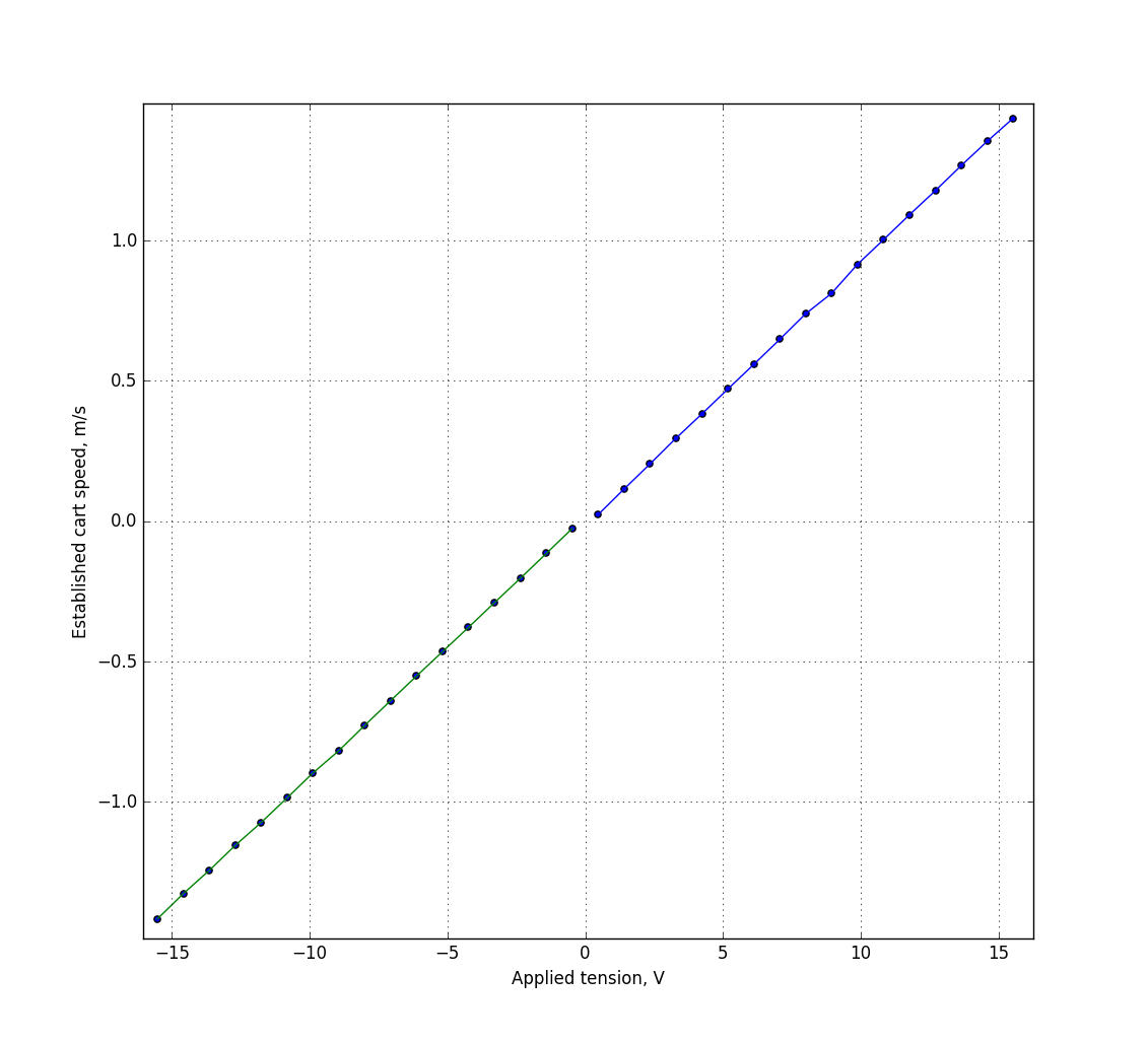
If I had no friction in the system, then this graph would be linear, and my model would be constructed as v_ {k + 1} = a * v_k + b * u_k. And after all, it is almost linear in its positive and negative parts at the same time, but these two straight lines do not pass through zero. This is (including) due to friction. We see that if at a positive voltage we add, and at a negative we literally take a fraction of a volt, the graph will pass through zero and become linear.

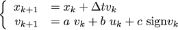
If we want to take into account the friction in the system, then the model is constructed as follows (do not forget to read the previous article, if it is not clear where this formula comes from):



So, with the data, we need to find the values ​​of a, b, and c. Fitting can be done as you please, given that it is done only once on the desktop, you can simply make three nested cycles. Here is the fitting code that tells me that for a 20ms sampling between measurements, a = .4, b = .06, c = -. 01. That is, the voltage required to compensate for friction in my system is equal to one tenth of a volt. The curves obtained by this approximation are superimposed on the real measurement in the picture above.

We control the applied force, not the voltage

Total, at the moment our system can be written as follows:



Unfortunately, this is not a linear differential equation of the form x_ {k + 1} = A x_k + B u_k, which is necessary for a linear-quadratic regulator. In addition, even if it were not for this, then I need to add another pendulum to the carriage, but I do not know how to derive the dependence of the position and angular velocity of the pendulum on the voltage. I would prefer that, as a control, I would have not the tension, but the acceleration of the carriage itself:



Strictly speaking, x_ {k + 1} = x_k + dt v_k + (dt) ^ 2/2 a_k, but for dt = .02 seconds (dt) ^ 2/2 equals .0002, which is already negligible, therefore discarded from records

OK, suppose my regulator uses acceleration as a control. But in fact, in reality, I have to apply voltage to the motor. How to get it? Very simple:



That is, having the current speed (system state), we can easily calculate the voltage that must be applied to obtain the necessary acceleration. Thus, we killed two birds with one stone at a time: and we got rid of the nonlinearity in the regulator, but at the same time leaving the friction compensation, and got an intuitive control. It is much easier for me to imagine acceleration rather than voltage, which has a very non-linear effect on speed.

Simple but long math or add a pendulum

Equations of motion of a pendulum

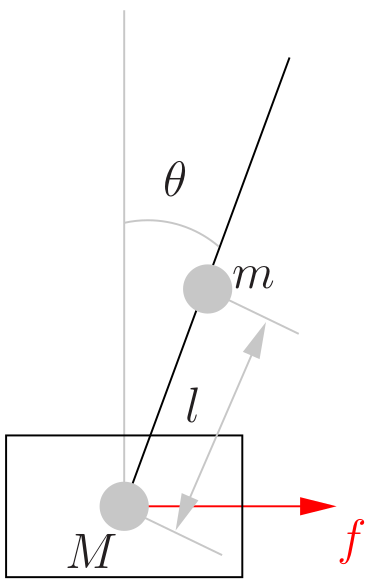
So, the task is to add a pendulum to our system and write the corresponding linear equations for the controller. Let's give a complete list of the necessary physical quantities for this:

• m: mass of the pendulum
• M: carriage weight
• f: force applied by the motor to the carriage through the belt
• 2l: pendulum length (l is the distance from the loop to the center of mass of the pendulum)
• I: moment of inertia of the pendulum (by the way, do your fonts allow you to see the difference between I and l?)
• θ (t): the angle of deflection of the pendulum from the vertical, zero in the unstable equilibrium position, increases clockwise
• x (t): carriage position

In total, the variables of my system will be a four-dimensional vector consisting of the position of the carriage, its speed, the angle of deflection of the pendulum and its angular velocity. The task now is to write a system of linear differential equations of this kind:



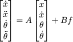
If we manage to record it in continuous form, then we simply discretize and we won the fight. Please note that here I use as a control the applied force, not acceleration, but Newton's second law will show us how to do this. So, we need to find the unknown matrices A and B.

Let us write Newton's second law for the carriage: the acceleration of the carriage multiplied by the mass equals the sum of two horizontal forces: the first force is our control, the force applied through the belt by the electric motor. The second force is the force with which the pendulum, trying to fall or rise, pushes the carriage to the side. To find it, we can write the coordinates of the center of the mass of the pendulum as a two-dimensional vector (x (t) + l sin (θ (t)), l cos (θ (t))). If we differentiate twice the coordinate, we get acceleration, and the force is the acceleration to the mass. Since we are only interested in the horizontal component, it makes sense to take only the second derivative of x (t) + l sin (θ (t). Total:



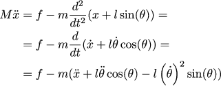
This is a non-linear equation, but it can be well approximated linear around an equilibrium point. If the angle is close to zero, then the first remarkable limit (well, or the Taylor series) says that the sine of the angle is approximately equal to the angle. The same for cosine: for angles close to zero, the cosine is almost equal to one. Well, in the same way, we neglect the powers, starting with the square (if we have a speed equal to .1 radians per second, then the square of the speed will give a very small contribution (.01), so we ignore them boldly):



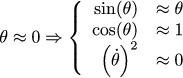
Then the previous equation can be approximated linear:



Now we write Newton's second law (version for rotation) for the pendulum. For a start, what is Newton's second law for rotation? This sum of the moments is equal to the angular acceleration multiplied by the moment of inertia. The moment of inertia is such an analogue of mass for translational motion. We are interested in the projection of all forces on the straight line, perpendicular to the pendulum (after all, only the perpendicular component rotates, right?) Well, of course, these forces must be multiplied by the shoulder to get a moment. The forces acting on the pendulum are three: gravity and the horizontal and vertical components of the support reaction force, which we can get as last time, twice taking the time derivative of the coordinates of the center of mass of the pendulum:



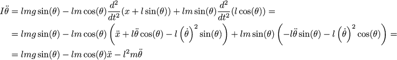
Let's approximate it with a linear equation:



We write equations (1) and (2) into the system:



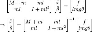
For convenience, we call the determinant of the matrix the letter D:



Let's reverse the matrix:



Now we write our differential equations, in fact, we found the matrices A and B:

Discretize the linear system

So, we have written the continuous differential equation:



For a constant step Δt we get the following:



If we denote by E the unit matrix 4x4, then we can write:



The moment of inertia for a rod that rotates around the end can be viewed here , so we simplify everything you can:



This is the most important equation of motion of the pendulum.

Line square controller

The code for calculating the coefficient of the regulator can be found here. I used to use the smallest squares for counting, but it is still rather cumbersome, so in the new code the gain matrix is ​​considered directly. Matlab for this is optional, quite enough for the usual python.

So, LCR, we are told that if we take the controlling force f_k = 24.95 x_k + 18.54 v_k + 70.44 θ_k + 14.96 ω_k, then we should get the following behavior systems:



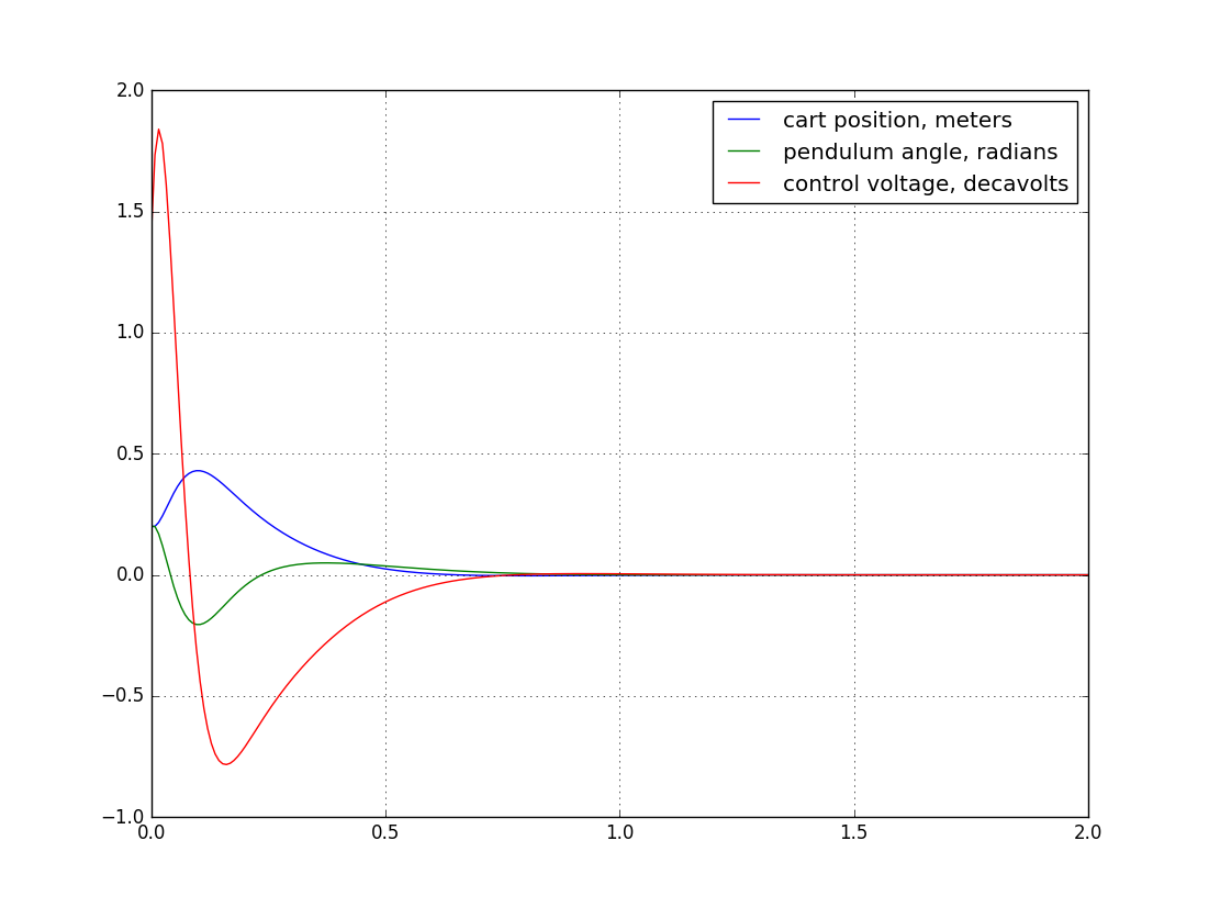
x_k is the position of the carriage, v_k is its speed, θ_k is the angle of the pendulum, ω_k is its angular velocity. The voltage on the graph is given in tens of volts to roughly equalize the scales of the three graphs.

We score coefficients in arduin

This is how I got a pendulum, the control code can be viewed here :



In principle, I am quite pleased with the result so far. The amplitude of the deviation of the carriage from the desired position in the area of ​​two centimeters, which is pretty decent. Why does it not stand still rooted to the zero position, catching the deviations of the pendulum with very small movements? There are several reasons. The simplest is a gap in the gearbox of the motor, which is about five millimeters of the carriage position, which means that the carriage is quite expensive to change the direction of movement. The next, and no less important reason is the estimate of the angular velocity of the motion of the pendulum (and of the velocity of the carriage).

How to estimate the speed of movement, if only an incremental encoder is available? The easiest way is to take the last two values ​​of the encoder and divide their difference by the past tense. This is known as finite differences and is widely used in practice.

Let's look at the following chart:



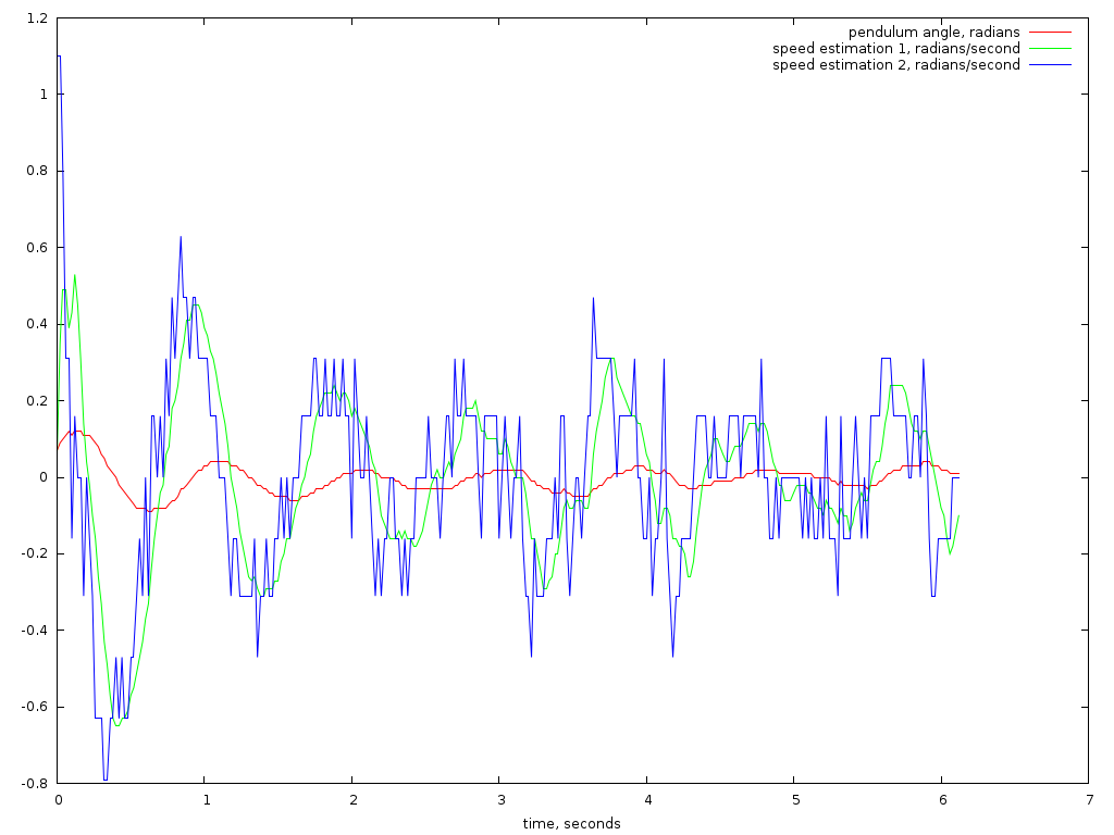
I recorded the angle of the pendulum for a few seconds, it is shown in red. The graph is a bit noisy due to the resolution of the encoder, but overall it’s pretty smooth. The speed we have to find synthetically from the history of the position of the pendulum. If we take directly the difference of two neighboring positions and divide by 20 milliseconds, then this will give us a blue graph. The advantage of finite differences is that they are very easy to program. Their disadvantage is that they dramatically amplify any measurement noise.

If we take this estimate of speed, then the regulator goes crazy:



The only difference with the previous video is the speed rating, nothing else.

In an amicable way, one would need to approximate the red curve by some polynomial, and assume its derivative is the main idea of ​​the Savitsky-Golay filter . In order not to rack my brains, I simply smoothed the speed estimate, taking not the next samples, but the difference of the current sample and eight samples ago, dividing by (20ms * 8). This approach greatly smoothes the speed estimate, but its disadvantage is that it lags the system. Look at the green curve: it is clearly behind the real situation. Such a delay in the estimation makes my pendulum sway slightly.

By the way, if you take the Savitsky-Golay filter in the forehead, it will also create a similar delay. Thus, I found a reasonable compromise for me between achieving the goal and the simplicity of artillery. I plan to deal with noisy measurements with completely different methods, this is a topic for future conversations. Also in subsequent conversations will include the automatic swing of the pendulum, so that he himself rises from the lower to the upper state.

Stay tuned!