Lossless data compression algorithms: what they say about markets

In our blog on Habré, we not only consider various technologies of the financial market, but also describe various tools used by analysts in the course of its analysis. In particular, not so long ago we wrote about how the hypothesis of random walk can be used to predict the state of the financial market. NMRQL quantitative analyst hedge fund Stuart Reed published on the website of Turing Finance, where he applied this hypothesis to test the randomness of market behavior.

The idea was as follows: random number generators are “run” through the NIST test group in order to understand where a vulnerability arises that makes it possible to use market inefficiencies for profit. In the course of the experiment, the author came to the conclusion that the behavior of the market cannot be described in terms of just tossing a coin, as certain authoritative scientists believe. Some tests were able to fix a certain level of "noise" in the market behavior. One of them, the linear complexity test, attracted the author's attention, because it recalls the idea of a relationship of chance and degree of compression.
')
In a new article, Reed tried to figure out the benefits that data compression algorithms can bring to the task previously set. We present to your attention an adapted translation of this work.

Market efficiency and the random walk hypothesis

In its extreme expression, the market efficiency hypothesis states that all information, whether public or privately available, is instantly and accurately taken into account in the value of the price. Therefore, any price forecast for the next day should be based on the current state of the market, since the current quotes correctly and fairly reflect the current state of affairs.

According to this theory, no detailed economic or fundamental analysis of the past will provide a more accurate forecast for the future. On the effective market from the point of view of completeness and sufficiency of information, the future is not defined, because it depends on unknown data that will appear “tomorrow”. Based on the position of today's observer, future changes are random. Only analysts who are able to travel in time can “crack” the market.

This hypothesis has its advantages, even if we stand for a more complex understanding of the situation, for the influence of evolutionary and behavioral factors. The merits of this theory are undeniable. Firstly, it is really difficult to predict the behavior of markets. Secondly, there really is no sequence of actions according to which the average player is able to hack the market. Thirdly, the efficiency hypothesis quite logically explains the emergence of such financial innovations, such as, for example, derivatives.

The most serious criticism of the effectiveness hypothesis comes from the behavioral financial analysis, which casts doubt on its fundamental postulates. As part of this approach, it is argued that investors do not behave rationally and are not able to give a “fair” price to shares. Players in practice do not have uniform expectations about the price.

The evolutionary theory of market development adds a couple more arguments to this. She believes that the system consists of disparate agents that interact with each other, subject to evolutionary laws. In this interaction, accident, momentum, cost and turnover of assets (reversion) come to the fore. None of these evaluation criteria prevails over the others. Their impact on market conditions changes as players adapt to their effects. The efficiency hypothesis calls such things market anomalies, which is not entirely true. Their appearance is quite predictable, and the impact on the market can be quantified.

In response to criticism, market efficiency advocates developed two new hypotheses. One claims that only public information is reflected in the quotes. The other goes so far as to recognize the influence of historical data on current stock prices. But the main position remains the same: the price movement follows the distribution of the Markov chain, random walk.

It turns out that we duplicate the random walk hypothesis underlying almost all modern price models. Academics and market practitioners have spent decades studying the relative effectiveness and randomness of markets. In the last article, Stuart Reed presented one of the tests for randomness testing - the heterogeneous dispersion relation test of Law and McKinley. This time, among other things, we will discuss the Lempel-Ziv compression algorithm.

Algorithmic Information Theory and Accident

For quantitative analysis, the study of chance is not new. This has long been engaged in cryptography, quantum mechanics, genetics. It is not surprising that some ideas and approaches were borrowed from these sciences. For example, from an algorithmic information theory, economists have taken the idea that a random sequence is incompressible. Let's first try to set the context for this interesting thought.

In the 1930s, Alan Turing presented an abstract model of computing, which he called an automatic machine. Today it is known as the Turing machine. In this regard, we are only interested in the following statement: “It doesn’t matter what algorithms of computation are laid, the machine should imitate the logic of the algorithm itself”

Turing machine model

In its simplified form, the algorithm is a deterministic sequence of steps for transforming an input data set into an output set. For a sequence of Fibonacci numbers, such an algorithm is easy to construct: the next number is the sum of the two previous ones. According to another great mathematician Andrei Kolmogorov, the complexity of a sequence can be measured in terms of the length of the shortest computational program, which generates this sequence as an output. If this program is shorter than the original sequence, then we squeezed the sequence, that is, coded it.

What happens when we put a random sequence S in the Turing machine? If there is no logic in the distribution of data, the machine has nothing to simulate. The only option to get a random sequence at the output is print S. But this program is longer than the random sequence S. Therefore, by definition, its complexity is higher. This is what they mean when they say that a random sequence is incompressible. Another question is, how can we back up the fact that the program we found is the shortest possible? In order to come to this conclusion, we should go through an infinite number of combinations.

Simply put, Kolmogorov’s complexity is not computable. Consequently, randomness is not computable. We cannot prove that the sequence is random. But this does not mean that we are not able to test the possibility that the sequence may be random. This is where statistical randomness tests come into play, some of which use compression algorithms.

Compression and market randomness: problem statement

Only a few scientists tried to adapt the compression algorithms to test the effectiveness of the markets. The idea itself is simple, but behind this simplicity are specific challenges.

Challenge 1: finite sequence and infinity

Our definition of randomness in the information theory means that we have to deal with infinite length. Any final sequence may be slightly compressed based on probability alone. When we use compression to test relatively short sequences in the market, we don’t care if the algorithm is able to compress them. We wonder if the level of compression will be statistically significant.

Challenge 2: Market Drift

There are several types of randomness. The first type is called martingale or real Kolmogorov randomness. It is most often associated with computer science and information theory. The second type is Markov's randomness, used in financial analysis and the random walk hypothesis.

This means that we must be extremely careful when we choose a statistical test for market randomness. The statistical test developed for the first type of randomness will have a confidence interval different from that of the test for Markov's randomness.

It should be a little cleared up now. Suppose we have two models: Brownian motion and geometric Brownian motion with non-zero deviation. In our example, the first model is suitable for both types of randomness. The second only for Markov's chance. The test result of the second model will be distorted.

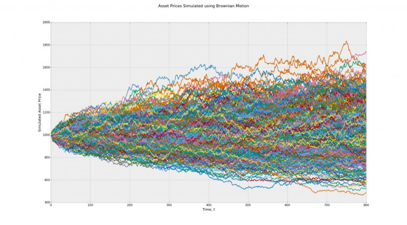
Model 1 (Brownian motion) - on average, all paths lead nowhere, with zero deviation. With binarization, this model turns into a coin flip sequence.

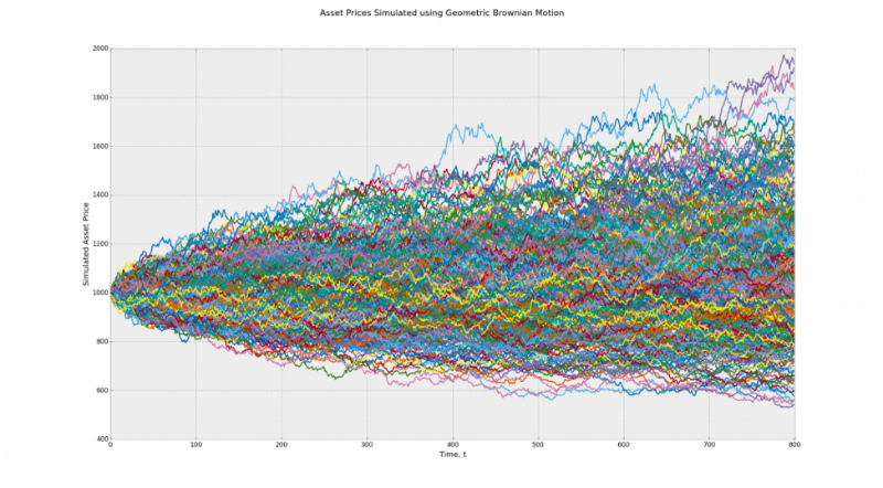
Model 2 (Geometric Brownian motion) - the paths lead up, and the deviation is non-zero. When binarization results will be distorted

This is a serious problem for those who want to disprove the random walk hypothesis through compression. Since the theory deals only with excessive predictability of market drift, that is, the ability of someone to crack the market.

Challenge 3: stochastic volatility and breaks

The next problem is that the non-stationarity of volatility can lead to the fact that certain market movements will look like regular and frequent phenomena contrary to theoretical calculations. This problem is also called "fat tails." If we assume that the noise of market changes tends to zero, regardless of gaps and stochastic volatility, we can imagine changes in the binary code and remove the problem.

Compression test for market randomness

In academic science, lossless data compression algorithms have already been used in relation to the assessment of market efficiency. The essence of most studies is as follows: developed markets demonstrate a high level of efficiency, emerging markets show excessive compressibility and a certain level of inefficiency. These inefficiencies can only be explained through specific patterns that indicate a level of probability higher than expected at certain time intervals.

Verification methodology

The methodology is based on three known compression algorithms: {gzip, bzip2 and xz}.

You need to download market indices from Quandl.com.
Then calculate the logarithmic returns of the indices and designate them as r.
Calculate their average (deviation component) - μ _r .
To remove the directivity (detrend) r μ _{r is} read from it.
Then r is transferred to the binary system, replacing values greater than zero by one, and values less than zero, respectively, by zero.
Then r is divided into m through the imposition of discrete windows - W for 7 years each.
Each window is converted to hexadecimal wh (4-day sub-sequence).
Each w _h , w _hc is compressed and the compression ratio is calculated .
This average is distributed across all windows - c ^∗ .
The expected compression ratio is calculated using pseudo-random data - E [c ∗].
If c ^∗ > = min (1.0, E [c ^∗ ]), the market does not exhibit excessive compressibility, which implies its effectiveness.
If c ^∗ <min (1.0, E [c ^∗ ]), then excessive compressibility is present, which implies market inefficiency.

R test and algorithm parsing

On R it took not so much code to do such a test, since it already has the functions memCompress and memDecompress. Similar functions exist in Python.

compressionTest <- function(code, years = 7, algo = "g") { # The generic Quandl API key for TuringFinance. Quandl.api_key("t6Rn1d5N1W6Qt4jJq_zC") # Download the raw price data. data <- Quandl(code, rows = -1, type = "xts") # Extract the variable we are interested in. ix.ac <- which(colnames(data) == "Adjusted Close") if (length(ix.ac) == 0) ix.ac <- which(colnames(data) == "Close") ix.rate <- which(colnames(data) == "Rate") closes <- data[ ,max(ix.ac, ix.rate)] # Get the month endpoints. monthends <- endpoints(closes) monthends <- monthends[2:length(monthends) - 1] # Observed compression ratios. cratios <- c() for (t in ((12 * years) + 1):length(monthends)) { # Extract a window of length equal to years. window <- closes[monthends[t - (12 * years)]:monthends[t]] # Compute detrended log returns. returns <- Return.calculate(window, method = "log") returns <- na.omit(returns) - mean(returns, na.rm = T) # Binarize the returns. returns[returns < 0] <- 0 returns[returns > 0] <- 1 # Convert into raw hexadecimal. hexrets <- bin2rawhex(returns) # Compute the compression ratio cratios <- c(cratios, length(memCompress(hexrets)) / length(hexrets)) } # Expected compression ratios. ecratios <- c() for (i in 1:length(cratios)) { # Generate some benchmark returns. returns <- rnorm(252 * years) # Binarize the returns. returns[returns < 0] <- 0 returns[returns > 0] <- 1 # Convert into raw hexadecimal. hexrets <- bin2rawhex(returns) # Compute the compression ratio ecratios <- c(ecratios, length(memCompress(hexrets)) / length(hexrets)) } if (mean(cratios) >= min(1.0, mean(ecratios))) { print(paste("Dataset:", code, "is not compressible { c =", mean(cratios), "} --> efficient.")) } else { print(paste("Dataset:", code, "is compressible { c =", mean(cratios), "} --> inefficient.")) } } bin2rawhex <- function(bindata) { bindata <- as.numeric(as.vector(bindata)) lbindata <- split(bindata, ceiling(seq_along(bindata)/4)) hexdata <- as.vector(unlist(mclapply(lbindata, bin2hex))) hexdata <- paste(hexdata, sep = "", collapse = "") hexdata <- substring(hexdata, seq(1, nchar(hexdata), 2), seq(2, nchar(hexdata), 2)) return(as.raw(as.hexmode(hexdata))) }

GitHub Code

The following is a brief description of the three compression schemes used in the compression algorithm.

Gzip compression Based on a DEFLATE algorithm that combines LZ1 and Huffman encoding. LZ1 is named for Abraham Lempel and Jacob Ziv. It works by replacing repeating patterns in a sequence, placing links to copies of these patterns in the original uncompressed version. Each match is encoded through a long pair containing the following information for the decoder: the parameter y is equal to all parameters through the distance x after it. The second algorithm, named after David Huffman, constructs the optimal prefix tree by the frequency of occurrence of patterns in the sequence.
BZIP2 compression . Uses three compression mechanisms: the Burrows-Wheeler transform, the start-to-front (MTF) transform, and the Huffman coding. The first of these is the reverse method for rearranging the sequence into a stream of similar characters to simplify the compression procedure using standard methods. The MTF transform replaces the letters in the sequence with their indexes on the stack. Thus, a long sequence of identical letters is replaced by a smaller number, rarely found letters - by a larger one.
XZ compression . Works through a sequence of algorithms Lempel-Ziv-Markov, which was developed in 7z compression format. This is, in essence, a vocabulary compression algorithm that follows the LZ1 algorithm. Its output is encoded using a model that performs a probabilistic prediction of each bit, called an adaptive binary range encoder.

All three algorithms, for example, are available in the R language through the memCompress and memDecompress functions. The only problem with these functions is that the input must be given in hexadecimal sequence. For translation you can use the function bin2rawhex.

Results and their o (demon) meaning

For the experiment used 51 global market index and 12 currency pairs. The sequences were tested for weekly and daily frequency.

All assets were compressed using gzip, bzip2, and xz algorithms using the walk-forward methodology. With the exception of the dollar / ruble pair, none of the assets showed excessive compressibility. In fact, none of them showed any compressibility at all. These results confirmed the conclusions of the past experiment with a linear complexity test. But they contradict the results of the NIST tests and the results of the Lo-McKinley test. It remains to figure out why.

Option 1. The first conclusion is to recognize (to the delight of academicians) that world markets are relatively effective. Their behavior looks quite random.

Option 2. Or you can admit that there is definitely something wrong with the compression algorithms without losing data in terms of checking the effectiveness and randomness of financial markets.

To test these hypotheses, the experiment author had to develop a test to test the compression test.

Compression Test

Opponents of the random walk hypothesis, in fact, do not insist on 100% determination of markets. The point is to prove that the behavior of the markets is not 100% random. In other words, markets have two aspects: signal and noise. The signal manifests itself in hundreds of anomalies, and the noise acts as an obvious coincidence and efficiency. These are two sides of the coin. The next step is to recognize that the noise produced by the system does not cancel the effect of the signals. It remains possible to "hack" the market, finding and using such signals.

Based on the above, the author proposes the following formula for testing the compression test:

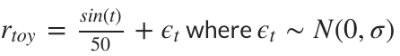
If we increase the size of the standard deviation of the noise component - ϵt, we observe how the compressibility of the market begins to deteriorate. When the standard deviation passes the 0.01 mark, the compression test begins to fail:

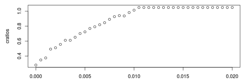
Examples of conclusions in the test for σ = 0.010, σ = 0.020 and σ = 0.040 are as follows:

In the compression test, all these markets are random or effective, because they cannot be compressed through data lossless compression algorithms. Yes, they may seem random. But they consist of signals and noise, so the accident can not be complete.

For a more adequate test, it is necessary to use a betting strategy / algorithm for returning to the average:

Conclusion: window size w = 4;
For the time parameter t, we calculate the cumulative return to the past w-minus day t - c.
If c <0.0, we retain 100% of the asset (we put on the fact that the asset goes up);
In any other case, throw off the stock.

Below are two charts for each noise level. The first one presents 30 stock curves generated by the rate return to average strategy. The second shows the average market income from the previous example compared to the income from the strategy.

This is a simplified example, but it helps to reveal a contradiction:

If the market is not compressed, it follows from this that it is effective, but if it were truly effective, it would have been impossible to apply a betting strategy to it that “hacks” it.

We have to “understand and forgive” because chance is unprovable, the sequence is not actually random. According to the author, the compression test failed because it is more sensitive to noise than the trading strategy (in the simulation it gives a 10-fold sensitivity to noise). The reason may be in the use of compression algorithms without data loss.

The code for the verification test can be viewed here .

findings

This study presented the idea of how to test the randomness of markets with the help of compression algorithms, and what it does to understand their effectiveness. Then a “metatest” was launched, which indicated the high sensitivity of such tests to any noise. As a result, we can draw several conclusions:

After detrending, the market begins to show enough noise and becomes “impassable” for data lossless compression algorithms (gzip, bzip2, and xz).
If the sensitivity of the test to noise is higher than that of the trading strategy (in the example of the article, such a test was 10 times more sensitive to noise than a simple betting strategy), a negative result does not mean that the analyzed market is effective. In the sense that it can not be "hacked."
In other words, such tests do not prove the correctness of academicians who insist on a rigid interpretation of the random walk market hypothesis. It just came out harder than it seemed at first glance.
Statistical tests to determine the randomness of the market vary in size, coverage and sensitivity. A reliable result can only give a combination of several tests.