Meduza.io: what about the likes?
Once, while reading the news on Medusa, I noticed that different news has a different ratio of likes from Facebook and VKontakte. Some news is megapopular on fb, and other people are shared only on VKontakte. I wanted to look at this data, try to find interesting patterns in them. Interested invite under the cat!
Data scraping
The first thing you need to get data for analysis. Anticipating the imminent release of Python + BeautifulSoup, I began to read the source code of the pages. The disappointment waited pretty quickly: this data is not loaded immediately with html, but deferred. Since I do not know how to javascript, I started looking for legs in the network connections of the page, and rather quickly came across a wonderful jellyfish API handle:
https://meduza.io/api/v3/social?links=["shapito/2016/05/03/poliem-vse-kislotoy-i-votknem-provod-v-rozetku"] The handle returns a nice looking json'ku:

And of course, since links is an array, I immediately want to try to substitute several records there at once, and, hooray, we get the list of interest.
I didn't even have to parse!
Now I want to get information about the news itself. Here I would like to thank the sirekanyan barn for his article , where he found another pen.
https://meduza.io/api/v3/search?chrono=news&page=0&per_page=10&locale=ru Experimentally it was possible to establish that the maximum value of the per_page parameter is 30, and about 752 page at the time of this writing. An important test that the social handle will withstand all 30 documents, passed successfully.
It remains only to unload! I used a simple python script
stream = 'https://meduza.io/api/v3/search?chrono=news&page={page}&per_page=30&locale=ru' social = 'https://meduza.io/api/v3/social' user_agent = 'Mozilla/5.0 (Windows NT 6.1; WOW64) AppleWebKit/537.36 (KHTML, like Gecko) Chrome/47.0.3411.123 YaBrowser/16.2.0.2314 Safari/537.36' headers = {'User-Agent' : user_agent } def get_page_data(page): # ans = requests.get(stream.format(page = page), headers=headers).json() # ans_social = requests.get(social, params = {'links' : json.dumps(ans['collection'])}, headers=headers).json() documents = ans['documents'] for url, data in documents.iteritems(): try: data['social'] = ans_social[url]['stats'] except KeyError: continue with open('res_dump/page{pagenum:03d}_{timestamp}.json'.format( pagenum = page, timestamp = int(time.time()) ), 'wb') as f: json.dump(documents, f, indent=2) Just in case, I substituted a valid User-Agent, but everything works without it.
Next, the script of my former colleague, alexkuku , helped me to parallelize and visualize the process. You can read more about the approach in his post , he allowed to do such monitoring here:

The data was downloaded very quickly, in less than 10 minutes, no captcha or a noticeable slowdown. Swung in 4 streams from one aypishnik, without any superstructures.
Data minining
So, at the output we got a big json'ka with data. Now pound it in the pandas dataframe, and twist it in Jupyter.
Load the necessary data:
df = pd.read_json('database.json').T df = df.join(pd.DataFrame(df.social.to_dict()).T) df.pub_date = pd.DatetimeIndex(df.pub_date) df['trust']=df.source.apply(lambda x: x.get('trust', None) if type(x) == dict else None) Build a boxplot
df[['fb', 'tw','vk']].plot.box(logy = True); 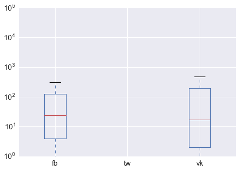
Just a few conclusions:
- Twitter has disabled the ability to watch the number of tweeted news. :-( We'll have to do without it.
- Distribution, as expected, is extremely abnormal: there are very strong outliers, which are noticeable even on the log scale (hundreds of thousands of reposts).
- At the same time, the average number of reposts turned out to be quite close: the median is 24 and 17 (here and below, facebook and VKontakte, respectively), the distribution vk is somewhat more "smeared".
So who are the most super-repostnuyu news jellyfish? Guess what?
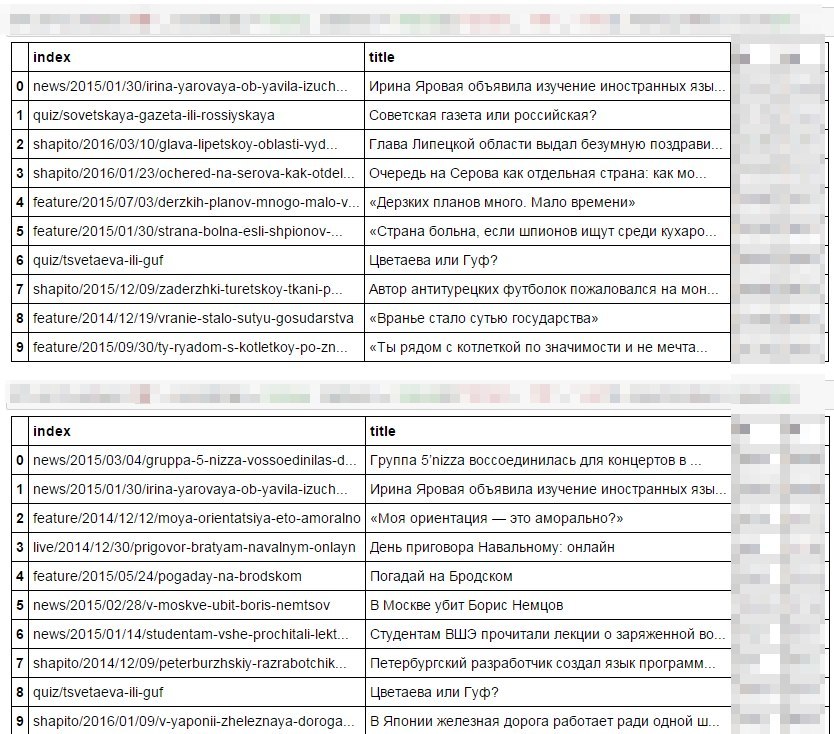
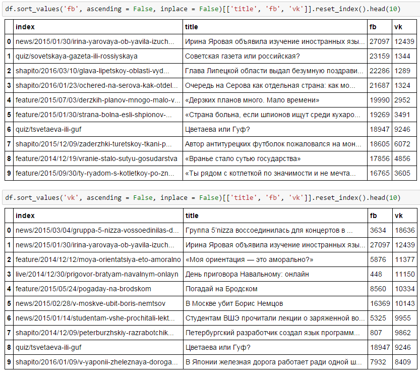
Well, of course, the first is FB: there are foreign languages, Soviet newspapers, Serov. And in the second 5nizza, "My orientation," the policy. I do not know how for me, so everything is obvious!
The only thing in which the preferences of the two social networks are similar: this is Irina Yarovaya, and yes Tsvetaeva with Guf.
Now, I want to look at the scatter plot of two quantities: the data is expected to correlate well with each other.
df['logvk'] = np.log10(df.vk) df['logfb'] = np.log10(df.fb) # sns.regplot('logfb', 'logvk', data = df ) 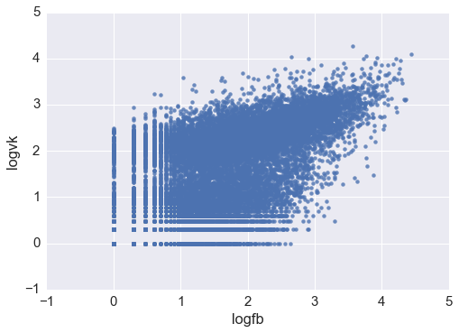
sns.set(style="ticks") sns.jointplot('logfb', 'logvk', data = df.replace([np.inf, -np.inf], np.nan).dropna(subset = ['logfb', 'logvk']), kind="hex") 
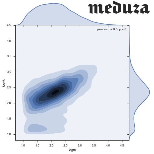
It seems, you can see two clusters: one with the center in (2.3, 2.4), and the second one smeared around zero. In general, there is no goal to analyze even low-frequency news (those that turned out to be uninteresting in social networks), so let's confine ourselves to recordings with more than 10 likes on both networks. Do not forget to check that we got rid of a small number of observations.
stripped = df[(df.logfb > 1) & (df.logvk > 1)] print "Working with {0:.0%} of news, {1:.0%} of social network activity".format( float(len(stripped)) / len(df), float(stripped[['vk', 'fb']].sum().sum()) / df[['vk', 'fb']].sum().sum() ) # Working with 47% of news, 95% of social network activity Density:
sns.jointplot('logfb', 'logvk', data = stripped, kind="kde", size=7, space=0) 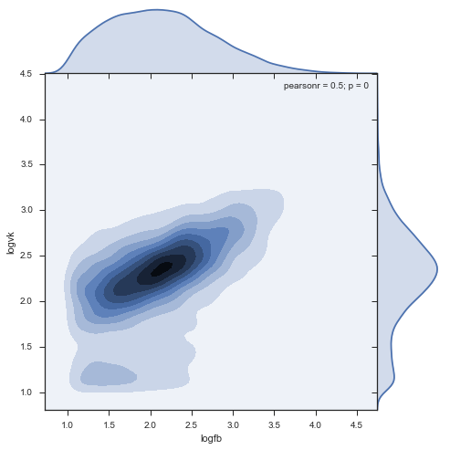
findings
- Found a dense cluster of commenting ratios: 220 on facebook, 240 on VK.
- The cluster stretches out more on facebook: in this social network, people repost more range, as compared to VC, where the peak is quite “narrow”
- There is a mini cluster of facebook activity at 150 fb and about 70 vk, quite unusual
Now I want to look at this relationship in dynamics: perhaps it has changed.
by_month = stripped.set_index('pub_date').groupby(pd.TimeGrouper(freq = 'MS')).agg({'fb':sum, 'vk':sum}) by_month.plot( kind = 'area') 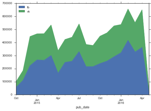
Interestingly, with a general increase in the volume of activity in social networks, Facebook is growing faster. In addition, there is not visible some kind of explosive growth, which I would expect to see in Medusa. The first months of activity was quite low, but by December 2014 the level had stabilized, the new growth began only a year later.
Let's look at the dynamics of the density distribution of comments from two social networks:
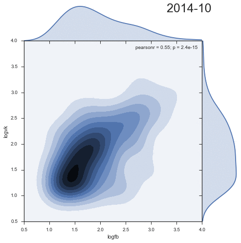
Quite entertaining that the second cluster decreases with time, and rather is an artifact of the past.
Finally, I want to check that the ratio of social networks does not change depending on the type of the document: Medusa has cards, stories, a tent, galleries, and also a training ground in addition to news.
def hexbin(x, y, color, **kwargs): cmap = sns.light_palette(color, as_cmap=True) plt.hexbin(x, y, gridsize=20, cmap=cmap, **kwargs) g = sns.FacetGrid(stripped.loc[::-1], col="document_type", margin_titles=True, size=5, col_wrap = 3) g.map(hexbin, "logfb", "logvk", extent=[1, 4, 1, 4]); 
In general, it is clear that the data is quite homogeneous by classes, there are no noticeable distortions. I would expect more social activity from the “tent”, but this effect is not observed.
But, if you look at the breakdown by the level of trust in the source , it’s nice to see that an unreliable source is less popular on social networks, especially on Facebook:

What's next?
On this my evening ended, and I went to sleep.
- I tried to teach a simple Ridle regression on word2vec data from article headers. You can look at the githaba , there is no special predictive power there. It seems that in order to predict the number of likes, it is worthwhile to at least train the model on the full news text.
- Based on these data, it is very good to catch the "bright" events that strongly stirred up the public. In this case, the ratio fb / vk can be a good predictor for the type of news.
- Social media activity now seems to be just as important a KPI for a newsman as is attendance. You can look at the authors / sources of popular posts, and on this base to evaluate the work. The contrast in the credibility of the source speaks in favor of this idea: false news is less posted on facebook. I think in one form or another this is already used in journalism.
')
Source: https://habr.com/ru/post/283058/
All Articles