Read more about the development of x-ray tomograph software
Scientists from Tomsk State University have created a microtomograph. The tomograph allows you to get to micron to learn about the internal structure of various materials, such as diamonds.
But it’s more interesting to stuff a fly into it.
')
The EDISON Software Developement was tasked to write software for the microtomograph. About how they successfully coped with the task, there was an article chookcha on Habré ( How to create software for a microtomograph for 5233 man-hours ) with a description of algorithms, mathematical methods, implementation and debugging.
Insatiable readers bombarded us with questions to which we finally formulated the answers ...
The tomograph can enlighten the material with a resolution of up to microns. It is 100 times thinner than a human hair. After scanning, the program creates a 3D model, where you can look not only at the outer side of the part, but also find out what's inside.
Video scan results
Tomograph device
List of the main technical characteristics of the device.
• Number of detector permitting elements: 2048 x 2018 cells with a size of one element of not more than 13.3 x 13.3 μm.
• Resolution: 13 microns.
• Overall dimensions: 504 x 992.5 x 1504 mm.
• Weight: 450 kg.
• Field of view: 1 mm.
• Operating wavelength range: 0.3–2.3 A.
• Accuracy of positioning of electromechanical motion modules in the PMT positioning system: ± 1 µm.
• Compliance with safety requirements: GOST 12.1.030-81.
• X-ray protection: 1–3 µSv / h.
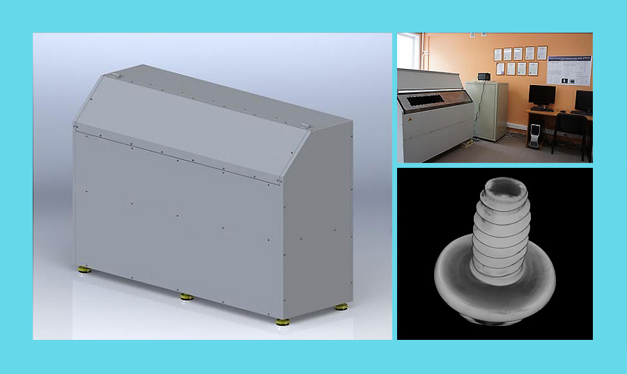
Fig. Appearance

Fig. The principle of operation of the electro-mechanical part
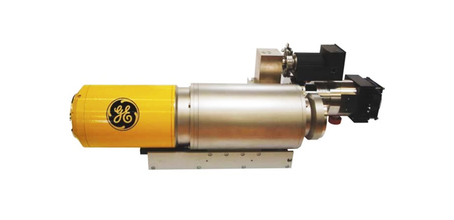
Fig. X-ray source
• Voltage: 20–160 kV.
• Current: 0–250 μA.
• Power: 10 watts.
• Diameter of focal spot: 1–5 microns.
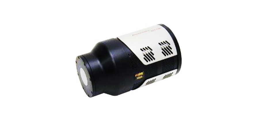
Fig. Positioning
• Rotor stroke: SAMD - 360 °, LEMD - 100 mm.
• Positioning accuracy, not less: ± 0.5 µm.
• The speed of the rotor: from 0.01 to 20 mm / s.
• Power: 0.7 kW at 70 V.
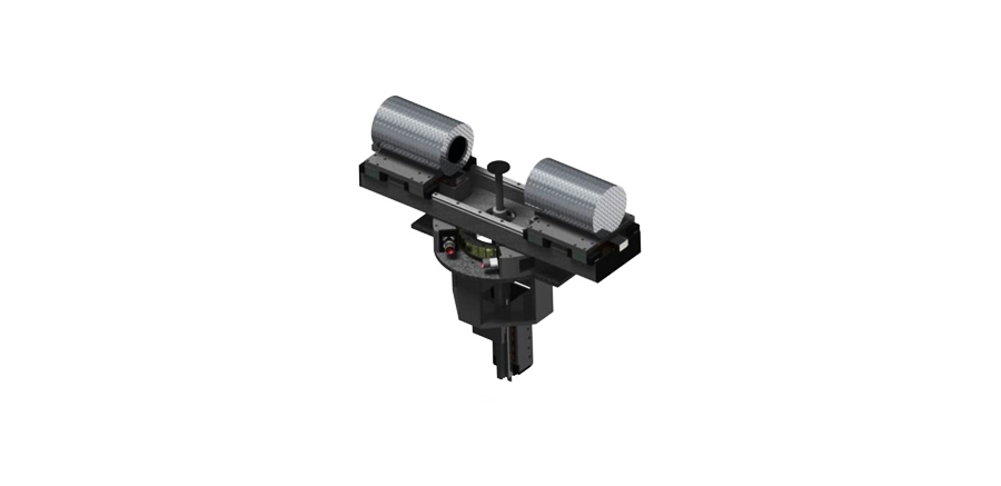
Fig. X-ray detector based on CCD
• Sensitive area of the CCD: 2048 x 2048 pixels.
• Geometrical pixel size: 13 x 13 microns.
• Geometrical size of the sensitive area of the CCD: 26.6 x27.6 mm.
• Built-in two-speed ADC: 16 bit, 100 kHz and 16 bit 2 MHz.
• Number of detector permitting elements: 2048 x 2018 cells with a size of one element of not more than 13.3 x 13.3 μm.
• Resolution: 13 microns.
• Overall dimensions: 504 x 992.5 x 1504 mm.
• Weight: 450 kg.
• Field of view: 1 mm.
• Operating wavelength range: 0.3–2.3 A.
• Accuracy of positioning of electromechanical motion modules in the PMT positioning system: ± 1 µm.
• Compliance with safety requirements: GOST 12.1.030-81.
• X-ray protection: 1–3 µSv / h.
Fig. Appearance
Fig. The principle of operation of the electro-mechanical part
Fig. X-ray source
• Voltage: 20–160 kV.
• Current: 0–250 μA.
• Power: 10 watts.
• Diameter of focal spot: 1–5 microns.
Fig. Positioning
• Rotor stroke: SAMD - 360 °, LEMD - 100 mm.
• Positioning accuracy, not less: ± 0.5 µm.
• The speed of the rotor: from 0.01 to 20 mm / s.
• Power: 0.7 kW at 70 V.
Fig. X-ray detector based on CCD
• Sensitive area of the CCD: 2048 x 2048 pixels.
• Geometrical pixel size: 13 x 13 microns.
• Geometrical size of the sensitive area of the CCD: 26.6 x27.6 mm.
• Built-in two-speed ADC: 16 bit, 100 kHz and 16 bit 2 MHz.
Question number 1
I would love to read about the conversion of the Radon transformation with a point source and about the implementation of this all using CUDA Uranix
Radon calculation for a point source, if schematically described, is similar to calculation for parallel mode, but only the direction of the rays is not parallel, which affects the coordinates of points in the object cube where the densities are added. With this schematic description, from the point of view of reconstruction, there is not much difference in which algorithm to use; only the coordinates of the segments / rays and the formula for calculating them change.
Further, when, based on the shadow projection, we received rays from the source to each projection point in the coordinate space of the microtomograph, knowing the position of the rotating cube of the object, voxels lying on the beam are calculated along each of the rays. Each voxel is assigned a pixel density value of the shadow projection into which the ray from the source enters, the data type of the scale is converted to float. As a result, for each shadow projection, we repeat this projection operation on voxels, taking into account the projection angle. After that, all the total voxel values are normalized to the bit depth in which they will be stored in the future, usually it was a 16-bit unsigned integer. This description explains in the most simplified way the scheme for reconstructing and obtaining the final voxel model, followed by a more detailed description of this algorithm.
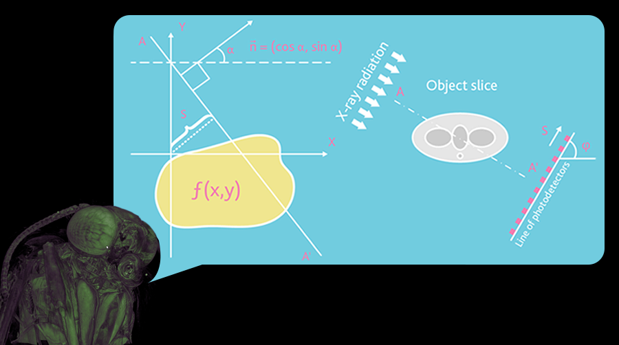
The X-ray system generates a flat shadow image of the complete internal volumetric structure of the sample, but in a separate shadow projection of the depth distribution of the structures of the sample are completely mixed. Only X-ray tomography allows visualizing and measuring the spatial structures of samples without their chemical and mechanical processing.

Fig. 1. Geometry of parallel beams
Any x-ray shadow image is a flat projection of a three-dimensional object. In the simplest case, we can describe it as an image obtained in parallel x-rays (Fig. 1). In this approximation, each point of the shadow image contains summary information on the adsorption of a particular X-ray beam over the entire volume of a three-dimensional object. For the parallel geometry of X-ray beams, the reconstruction of a three-dimensional image of a sample from a two-dimensional shadow projection is realized using a series of reconstructions of two-dimensional sections of the sample along one-dimensional shadow lines. The possibility of such reconstructions is demonstrated by a simple example: consider an object with a single point with high adsorption in an unknown place.

Figure 1.1. Schematic representation of the three different positions of the absorbing region and the corresponding reconstruction from the resulting shadow projections
In a one-dimensional shadow line, a decrease in intensity due to its absorption on the absorbent object will be observed (Fig. 2). Now we can simulate in computer memory an empty row of pixels (image elements) corresponding to the intended object displacement. Naturally, it is necessary to make sure that all parts of the reconstructed object will be in sight. Since we have the coordinates of the shadows from the absorbing areas of the object, we can select all possible positions of the absorbing areas inside the object as lines in the reconstructed area in the computer's memory. Now we begin to rotate our object and repeat this operation. In each new position of the object we will add to the reconstructed area lines of possible positions of the object in accordance with the position of its shadow projections. This operation is called reverse projection. After several turns, we can localize the position of the absorbing area inside the reconstruction volume. With the increase in the number of shadow projections from different directions, this localization becomes more and more clear (Fig. 3).

Fig. 2. Reconstruction of a point object using a different number of displacements
In the case of reconstruction, based on an infinite number of projections, an image is obtained with a good clarity of determining the position of the absorption region inside the object under study. At the same time, the dotted image will be accompanied by a blurred area, since it was obtained during the blending of lines with all possible deviations. Now, since we know that the image is formed by a point object, we can carry out a preliminary correction of the initial information in the sorption lines in order to make the final image more relevant to the real object. This correction adds a certain amount of negative adsorption along the outer edge of the point in order to remove the blurring inherent in the back projection process (Fig. 4). This algorithm provides not only images of sections of individual point structures, but also allows you to explore real objects. Each material object can be represented as a large number of individual elemental absorbing volumes and linear adsorption in each x-ray beam corresponds to the total adsorption on all absorbing structures encountered by the beam.

Fig. 3. Back projection filtering
Thus, two-dimensional sections of the object can be restored from one-dimensional shadow lines from different angles. However, most X-ray emitters are not capable of generating parallel beams of radiation. In reality, point sources are used to produce conical X-ray beams.

Fig. 4. Geometry of diverging beam
In the fan geometry, the reconstructed sections will have some distortions in areas remote from the optical axis of the beam. To solve this problem, we must use the algorithm of three-dimensional reconstruction of the conical beam (Feldkamp) to take into account the thickness of the object. In other words, the rays passing through the front and back surfaces of the object will not be projected onto the same row of the detector (Fig. 6). Thus, the most rapidly reconstructed section is the axial section, since it does not require a correction for the sample thickness.

Fig. 5. Geometry of a conical beam
In the case of fluoroscopy of the sample image contains information on the reduction of the intensity of the incident radiation inside the object. Since X-ray absorption is described by an exponential dependence (Lambert-Beer law), linear information on the adsorption of radiation from a shadow image can be disclosed using a logarithmic function. Since logarithm is a non-linear operation, the slightest noise in the signal leads to significant errors in the reconstructions. To avoid such errors, averaging of initial data can be used. On the other hand, we could try to improve the signal-to-noise ratio in the shadow image by optimizing the exposure time to accumulate the most representative information. The most effective way of noise reduction in the reconstruction process is the correct choice of the correction / filtering function for convolution before reverse projection. In the simplest case (described above), the correction function produces two negative adsorption reactions around any signal or noise peak in the shadow line, and this behavior becomes very dangerous when working with a noisy signal. The choice of correction for the function of convolution with spectral limitations (Hamming window) allows to solve this problem.
Job Description CUDA and Reconstruction
Reconstruction of shadow projection data
The maximum size of the cube for the reconstruction is 1024x1024x1024 voxels. Let's call such a cube unit. The algorithm allows to reconstruct smaller cubes, but at the same time the dimension in all directions should be a multiple of 32. For one approach, a cube layer is reconstructed, no more than 128 MB, i.e. 1/8 unit cube. If several CUDA devices are installed in the system, then the reconstruction will go on in parallel.
Shadow projections are loaded into RAM during the first pass, in an amount sufficient to reconstruct the cube. Those. if the reconstruction of the cube requires 1200 lines from the shadow projection, and the height of the file is 2000, then these 1200 lines of data from the file are loaded into RAM and cached. Since the reconstruction of the next cube, most likely, the projection segments will intersect, it will be possible to use the already loaded data again, reloading only new lines.
Server discovery and task distribution
UDP packets are used to locate clients and servers. At start and every 5 seconds the server sends such a notification. The client sends a broadcast request at the start, which forces the server to announce itself immediately. The client, having received a notification about the presence of the server, establishes a TCP connection with it, through which control commands, tasks are sent, and notifications about the completion of the task are received. All clients, servers, tasks have a unique identifier.
When you disconnect from one server, it is considered that the server has stopped and its tasks are redistributed among others. When a new server is connected, tasks from others are not selected or redirected to it. Therefore, for uniform loading it is important to find all the servers at the beginning of the distribution of reconstruction tasks. As the cubes are ready, it becomes possible to start merge tasks. Tasks are sent to a random server. Reconstruction and merge tasks are performed by servers in parallel.
Tasks can come from multiple clients. The server processes them in the order of receipt (FIFO). The client prefers to distribute reconstruction tasks from one layer of single cubes to one server in order to reduce the amount of data needed by the reconstruction server. The amount of RAM server determines the strategy for the reconstruction and compression of cubes. If there is a lot of memory (more than 20 GB), then the compression of the previous cube and the reconstruction of the next one are performed in parallel, otherwise the reconstruction of the next cube does not start until the cube is fully processed, i.e. compressed and saved to disk.
Basic reconstruction steps
First, the segments of the projections are determined, into which the reconstructed volume is projected taking into account the perspective. Based on these data, it is determined which projections are needed for reconstruction. If there are file segments in the RAM cache that are not included in this list, they are deleted from memory.
The reconstruction stream is cached by the projection segment, the memory block containing the projection (considering the page size of 4096 bytes) is locked in the memory, which prohibits its unloading into the swap, and the pointer is passed to the CUDA procedure. All further actions take place in the memory of the accelerator. There is a decompression of 12 bits in the float, then all calculations are carried out in the float. When unpacking, the segment is trimmed left and right to the width of the block being reconstructed, plus the gap required for convolution when filtering the projection. Pre-processing occurs: inversion, gamma correction, filtering by average projection, the required number of smoothing iterations. Next, a convolution occurs, and the segment is once again trimmed to the left and right to the minimum width necessary for reverse projection. This is how projections are processed, as long as there is enough memory on the video card. Those. on the video card, an array of segments is formed that are ready for back projection.
The essence of reverse projection is to sum up for each voxel from all projections the weight of the point from which the X-ray source beam hit. One call to the CUDA core calculates 32 voxels located one above the other. At the same time, a cycle is made for all projected segments loaded into memory. This allows you to store all intermediate data in registers and not to make intermediate entries in memory. At the end of the calculations, the density of the voxel is recorded in the memory. The back projection core has 2 implementations, one slow with checks that there is a point on the projection from which to take data, since there is not always a point at the ends of the projections where the value is taken from. The quick implementation performs no checks. The desired implementation is automatically selected. The sampling of the value from the projection is made by the “nearest neighbor” algorithm. The use of texture memory in the first stages showed a sharp decrease in performance, and at this stage when using arrays of projections, it was impossible to create texture arrays due to limitations of CUDA 4.2.
If there is not enough memory, then calculations may require several iterations of loading projections and back projection.
Upon completion of the calculations, the voxels are evaluated. The maximum and minimum density values are calculated, a histogram is constructed. The construction of the histogram and copying the results into RAM is performed in parallel.
If there are multiple CUDA devices, the segments of the reconstructed cube are processed in parallel. Upon completion of the cube reconstruction, another stream begins to engage in the compression of the cube, and the reconstruction flow is immediately taken to the next task, provided that there is enough RAM. As it turned out, the allocation and release of large memory segments is a very time-consuming operation; therefore, all received large blocks of memory are reused. So on CUDA memory allocation is made for a block of voxels, several intermediate buffers, and the rest of the memory will be allocated under the projection, and management of the placement of the projections in it is done manually.
Compression
Compression in the octree is made in several threads. The number of threads depends on the number of processor cores. Each thread processes its own octant. Then it is saved to the file that was specified by the reconstruction client in the task, and a notification is sent that the cube processing is completed.
Customer
The client maintains a database of cubes in the form of a SQLite file. It preserves the characteristics of cubes, the time of reconstruction, etc. Upon completion of the reconstruction, the client program is closed, thus it is possible to organize batch reconstruction tasks.
CUDA code sample
The kernel (measureModel.cu), which makes the first pass when calculating the histogram. The file is shown to show the general view of the code on CUDA in a real working project.
#include <iostream> #include <cuda_runtime.h> #include <cuda.h> #include <device_functions.h> #include "CudaUtils.h" #include "measureModel.h" #define nullptr NULL struct MinAndMaxValue { float minValue; float maxValue; }; __global__ void cudaMeasureCubeKernel(float* src, MinAndMaxValue* dst, int ySize, int sliceSize, int blocksPerGridX) { int x = blockDim.x * blockIdx.x + threadIdx.x; int z = blockDim.y * blockIdx.y + threadIdx.y; int indx = z * blocksPerGridX * blockDim.x + x; MinAndMaxValue v; v.minValue = src[indx]; v.maxValue = v.minValue; //indx += sliceSize; for (int i = 0; i < ySize; ++i) { float val = src[indx]; indx += sliceSize; if (v.minValue > val) v.minValue = val; if (v.maxValue < val) v.maxValue = val; } // __shared__ MinAndMaxValue tmp[16][16]; tmp[threadIdx.y][threadIdx.x] = v; // __syncthreads(); if (threadIdx.y == 0) {// 16 for (int i = 0; i < blockDim.y; i++) { if (v.minValue > tmp[i][threadIdx.x].minValue) v.minValue = tmp[i][threadIdx.x].minValue; if (v.maxValue < tmp[i][threadIdx.x].maxValue) v.maxValue = tmp[i][threadIdx.x].maxValue; } tmp[0][threadIdx.x] = v; } __syncthreads(); /// if (threadIdx.x == 0 && threadIdx.y == 0) { for (int i = 0; i < blockDim.y; i++) { if (v.minValue > tmp[0][i].minValue) v.minValue = tmp[0][i].minValue; if (v.maxValue < tmp[0][i].maxValue) v.maxValue = tmp[0][i].maxValue; } dst[blockIdx.y * blocksPerGridX + blockIdx.x] = v; } } void Xrmt::Cuda::CudaMeasureCube(MeasureCubeParams ¶ms) { // 256 int threadsPerBlockX = 16; int threadsPerBlockZ = 16; int blocksPerGridX = (params.xSize + threadsPerBlockX - 1) / threadsPerBlockX; int blocksPerGridZ = (params.zSize + threadsPerBlockZ - 1) / threadsPerBlockZ; int blockCount = blocksPerGridX * blocksPerGridZ; dim3 threadDim(threadsPerBlockX, threadsPerBlockZ); // dim3 gridDim(blocksPerGridX, blocksPerGridZ); MinAndMaxValue *d_result = nullptr; size_t size = blockCount * sizeof(MinAndMaxValue); checkCudaErrors(cudaMalloc( (void**) &d_result, size)); cudaMeasureCubeKernel<<<gridDim, threadDim>>>( params.d_src, d_result, params.ySize, params.xSize * params.zSize, blocksPerGridX ); checkCudaErrors(cudaDeviceSynchronize()); MinAndMaxValue *result = new MinAndMaxValue[blockCount]; checkCudaErrors(cudaMemcpy(result, d_result, size, cudaMemcpyDeviceToHost)); params.maxValue = result[0].maxValue; params.minValue = result[0].minValue; for (int i = 1; i < blockCount; i++) { params.maxValue = std::max(params.maxValue, result[i].maxValue); params.minValue = std::min(params.minValue, result[i].minValue); } checkCudaErrors(cudaFree(d_result)); } __global__ void cudaCropDensityKernel(float* src, int xSize, int ySize, int sliceSize, float minDensity, float maxDensity) { int x = blockDim.x * blockIdx.x + threadIdx.x; int z = blockDim.y * blockIdx.y + threadIdx.y; int indx = z * xSize + x; for (int i = 0; i < ySize; ++i) { float val = src[indx]; if (val < minDensity) src[indx] = 0; else if (val > maxDensity) src[indx] = maxDensity; indx += sliceSize; } } void Xrmt::Cuda::CudaPostProcessCube(PostProcessCubeParams ¶ms) { // 256 int threadsPerBlockX = 16; int threadsPerBlockZ = 16; int blocksPerGridX = (params.xSize + threadsPerBlockX - 1) / threadsPerBlockX; int blocksPerGridZ = (params.zSize + threadsPerBlockZ - 1) / threadsPerBlockZ; dim3 threadDim(threadsPerBlockX, threadsPerBlockZ); // dim3 gridDim(blocksPerGridX, blocksPerGridZ); cudaCropDensityKernel<<<gridDim, threadDim>>>( params.d_src, params.xSize, params.ySize, params.xSize * params.zSize, params.minDensity, params.maxDensity ); checkCudaErrors(cudaDeviceSynchronize()); } // #define DivideCount 8 #define ValuesPerThread 32 #define SplitCount 16 #define SplitCount2 64 __global__ void cudaBuildGistogramKernel( float *src, int count, int *d_values, int minValue, int barCount ) { // , int barFrom = threadIdx.x * ValuesPerThread; int blockIndx = SplitCount * blockIdx.x + threadIdx.y; int blockLen = count / (SplitCount * SplitCount2); unsigned int values[ValuesPerThread]; for (int i = 0; i < ValuesPerThread; i++) { values[i] = 0; } src += blockLen * blockIndx; for(int i = blockLen - 1; i >= 0; i--) { float v = src[i]; int indx = (int)((v - (float)minValue) * DivideCount) - barFrom; if (indx >= 0 && indx < ValuesPerThread) values[indx]++; } for (int i = 0; i < ValuesPerThread; i++) { d_values[blockIndx * barCount + barFrom + i] = values[i]; } } __global__ void cudaSumGistogramKernel( int *d_values, int barCount ) { // , int barIndx = blockIdx.x * ValuesPerThread + threadIdx.x; unsigned int sum = 0; d_values += barIndx; for (int i = 0 ; i < SplitCount * SplitCount2; i++) { sum += d_values[i * barCount]; } d_values[0] = sum; } void Xrmt::Cuda::CudaBuildGistogram(BuildGistogramParams ¶ms) { checkCudaErrors(cudaMemcpyAsync( params.h_dst, params.d_src, params.count * sizeof(float), cudaMemcpyDeviceToHost, 0 )); // int minValue = (int)(params.minDensity - 1);// , ! minValue = std::max(minValue, -200); // int maxValue = (int)params.maxDensity; maxValue = std::min(maxValue, 200); // ( 1 DivideCount ) int barCount = (maxValue - minValue + 1) * DivideCount; /// ValuesPerThread int x32 = barCount % ValuesPerThread; barCount += (x32 == 0) ? 0 : ValuesPerThread - x32; /// : /// x - 32 , .. x /// y - SplitCount dim3 threadDim(barCount / 32, SplitCount); /// , SplitCount2 dim3 gridDim(SplitCount2); /// SplitCount2 * SplitCount /// barCount / 32 /// int *d_values = nullptr; /// size_t blockValuesCount = SplitCount2 * SplitCount * barCount; size_t d_size = blockValuesCount * sizeof(int); checkCudaErrors(cudaMalloc( (void**) &d_values, d_size)); /// cudaBuildGistogramKernel<<<gridDim, threadDim>>>( params.d_src, params.count, d_values, minValue, barCount ); // GPU cudaSumGistogramKernel<<<dim3(barCount / ValuesPerThread), dim3(ValuesPerThread)>>>( d_values, barCount ); checkCudaErrors(cudaDeviceSynchronize()); // params.histogramValues.resize(barCount); checkCudaErrors(cudaMemcpy( ¶ms.histogramValues[0], d_values, barCount * sizeof(int), cudaMemcpyDeviceToHost )); checkCudaErrors(cudaFree(d_values)); params.histogramStep = 1.0 / DivideCount; params.histogramStart = (float)minValue; } Question number 2
The camera that you used (PIXIS-XF, presumably) gives 2048x2048 images, and in the article you write “up to 8000x8000”. This is how you got? Do you also move the sample or camera vertically and horizontally and then glue the pictures together? AndreyDmitriev
Yes, the PIXIS-XF: 2048B camera was used in the micro tomograph. The size of the reconstruction according to TK 8000x8000x20000, in width and depth of 8000 means that the camera sees only a part of the image, but it is reconstructed more, this gives a drop in the quality of the reconstruction at the edges. The table simply moves along the height, a new reconstruction is made, and the results are glued together.
Question number 3
The demo images that are in the video at the end of the article are all derived from 360 projections? If so, then it is good, because 360 projections with a step to a degree are quite a few, usually going with a third / quarter degree step, otherwise there will be reconstruction artifacts. It seems there is a formula for the optimal number of projections for a given resolution, but he forgot. AndreyDmitriev
In our case, 180-360 projections were used. Different algorithms can produce different quality of reconstructions depending on the number of projections, but in general the rule is that the quality increases with an increase in the number of projections. For our tasks, it was enough to use 180-360 projections to obtain good quality.
The algorithm normally reacts to frame drops at the cost of a small decrease in resolution in the direction where there are gaps. In addition, the camera had a peculiarity of overheating, and its “brightness” swam, therefore some of the frames were rejected as defective, the rest were normalized by the average brightness.
Question number 4
I also did not quite understand the frequency of the camera. According to the specification, it is dual-frequency at 100 kilohertz or two megahertz. If she has four megapixels, does this mean that she gives a frame every two seconds at the maximum frequency? AndreyDmitriev
Yes you are right.
According to the camera documentation , the frequency characteristics are as follows: ADC speed / bits 100 kHz / 16-bit and 2 MHz / 16-bit
That is, if one point of the image has a bit depth of 16bit, then we get that the frequency for the whole image will be: 2,000,000 / (2048 * 2048) = 0.47 hertz
Question number 5
Do you move the manipulator step by step or continuously? How long does it take to scan typical samples that are presented in the video? AndreyDmitriev
The manipulator (table) moves step by step. Turned to the corner, stopped, shot, turned again, etc.
The average scan time is 11 minutes per 378 frames.
Question number 6
Well, about 12 bits - very curious. The fact that cutting off four bits and packing every two pixels in three bytes is possible for storage and transmission is understandable. But for the reconstruction you also have to re-deploy each pixel of at least two bytes? Or do you have all the math on 12 bits? In this case, how did you solve the problem that the pixels occupy one and a half bytes and are not aligned to the border? AndreyDmitriev
The file format is 12 bit lateral projections.
- Pixels are packed bit by bit and arranged in rows, so that two points occupy 3 bytes, while it is assumed that the width of the projection image is a multiple of 2, according to the formula: lineWidthInBytes = width () * 3/2.
- Usually, the entire amount of data is not loaded immediately, but “windows” are used, in which only the necessary portion of the image is loaded, and the left and right borders are assumed to be a multiple of four pixels.
- After loading the “window”, further work is carried out using the functions of full import / export of this window into float or quint arrays. In the process of importing / exporting, a conversion from 12 bits to the required bit depth occurs.
- In our case, the gain from reducing the size of projection files was greater than the loss of performance in doing so. In addition, since the files were not completely loaded, but only the “windows” intended for processing on a specific cluster machine, the performance loss is even less due to the parallelization of tasks.
Volumetric (voxel) real-time rendering
Also interesting was the mapping of the model using voxels in real time. In addition to the voxels of the model itself, it was necessary to display in 3D such tools as the bounding box, the section plane, hide half of the object along the section plane, and also hide the object outside the box. On the cutting plane, the user interface element is displayed in the form of a “lever” (which at the same time corresponds to the normal vector), which allows you to move the projection slice window along the cutting plane and shift the plane itself along the normal vector. The projection slice window can also be stretched beyond its borders and rotated. On the bounding box, in addition to its edges, the same “levers” appear on the plane, which also allow you to change its dimensions. All these manipulations are performed in real time and the volume of the model space.
A sufficient frame rate during operation was provided due to the dynamic level of detail, since the data is loaded automatically when the bounding box is reduced.
For manipulation of interface elements in 3D, special sets of mathematical functions were implemented. The initial creation of a cutting plane, if described in general terms without using formulas, looks like this: the user double-clicks the mouse at any point of the model, after which this point is fixed and the normal vector to the created plane is displayed from it with further mouse movement. At the same time, the plane has already been created, and it lies on the ray coming from the screen coordinates of the mouse cursor into the space, not parallel to the perspective lines, so that the ray is projected as a point on the screen, and the orientation of the plane changes dynamically when the mouse is moved, immediately on the screen. To complete the creation, click once again to fix the orientation of the plane.
In addition to the elements of model manipulation, there are tools in the volume for controlling the color spectra of densities and levels of transparency.
Directly, the rendering of voxels and cropping with the cutting plane and the bounding box were implemented using the VTK library.
List of Math Functions
Mathematical classes and functions used for geometric calculations in the project.
1. Class plane .
- Description of the plane normal and point .
- Description of the three points .
- The angle of rotation of the 2D coordinate system inside the plane around the normal vector.
- Indenting the boundaries of a 2D rectangular area inside a plane with a reference point on the normal vector.
- The transition functions from a 2D point inside the plane rotated around the normal to real 3D coordinates and the inverse transform.
2. A set of mathematical functions for geometric calculations.
- Getting on the basis of the vector of two vectors mutually perpendicular and perpendicular to the original vector .
- Getting a vector perpendicular to this vector in a 2D coordinate system .
- Definition of an octant in the direction of a vector and vice versa creation of a vector in an octant.
- Correction of the center point of the plane for its positioning inside the bounding box.
- Check the entry point in the box.
- The intersection of the beam and the plane .
- The intersection of the segment and the plane.
- The distance of a point from a straight line .
- Perpendicular to the line from an arbitrary point to a point on the line .
- The distance from the point to the plane .
- The projection of the point on the plane .
- Projection of vector onto vector .
- Angle between 2D vectors .
3. Mathematical functions used in the reconstruction.
- Inversion.
- Gamma Correction .
- Filtering averaged projection.
- The required number of smoothing iterations .
- Convolution.

More projects:
How to create software for a microtomograph for 5233 man-hours
SDK for the introduction of support for e-books in FB2 format
Control access to electronic documents. From DefView to Vivaldi
Integrating two video surveillance systems: Axxon Next and SureView
Read more about the development of x-ray tomograph software
Sphere: how to monitor billions of kilowatt-hours
Developing a simple plugin for JIRA to work with a database
To help DevOps: a firmware builder for network devices on Debian for 1008 hours
Windows Service Auto Update for Poor AWS
Source: https://habr.com/ru/post/282848/
All Articles