The path of the laplacian. Part 2

And if we do not wipe on our Dijkstra Edsger?

In the first part, we described a method for ranking symmetrically related objects (nodes of an undirected graph) with respect to a given direction. For each object (node), the potential (Laplacian) is calculated, which determines its position relative to the specified source and target. In this article, we show how the potentials of the nodes simplify the task of finding the shortest paths (optimal routes). And also how the potentials themselves change when the external conditions change.

In the general case, the minimized value is not necessarily the distance, - the weights of the graph edges can be costs, fines, losses, times, - any values ​​that can be added. The task is a classic, the most simple algorithm for searching the shortest path was given by E. Dijkstra in 1959.

Flow map

On the basis of the potentials calculated in the previous part and the given connections / conductivities (inverse distances), a flow map can be drawn. Here is her view:
')

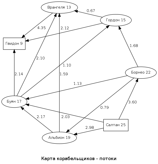
The source (Sultan) and the receiver (Guidon) are highlighted in squares. Next to the name of the node (island) is the rounded value of the potential. The numbers next to the arrows reflect the amount of flux (potential difference divided by the distance).

If Saltan had gone to Guidon as an army, he would have had to distribute the directions of movement of the masses, taking into account the magnitudes of the flows indicated on this map. Or if Sultan was a mosquito a photon or an electron - then he would also fly / swim in all ways at the same time. But in the real world, single-handed travelers with a non-zero mass rule, so we need not all the ways, but quite the opposite - one, but the best.

The presence of potentials simplifies (accelerates) the construction of the optimal path. There are two main algorithms - fast (but without guarantees of optimality) and precise. The latter is also fast (relatively classic), but slower than the first.

Algorithm Neo

Recall the recommendation of Neo - " if you want to get to the deadline, swim by the maximum flow ." We can use it on the basis of the given map.

The idea is this. For each node of the graph shown in the figure (except for the initial one), it is necessary to leave only the incoming branch and delete all the others. This ensures the unambiguous route from the source. The condition for selecting the incoming branch will be the maximum flow.
In order to ensure the speed of the algorithm and not go through all the nodes of the graph, we must start with the final (target) node and move from it along the branches with the maximum flow to the beginning.

According to the map, the maximum flow (4.35) to Guidon comes from Wrangel - it means that we leave the Wrangel-Guidon branch (we include it on the way).
We pass along the branch to Wrangel. The maximum flow to Wrangel (2.10) goes from Buyan - go to Buyan. From Buyan respectively to Albion, from Albion - to Saltan, the path is built. In our case, it is really optimal (relative to the weights of the branches of the original distance map) - lucky.

The advantage of this method is the simplicity and speed of construction of the path. We iterate only those nodes of the graph that are included in the route, that is, the speed of the algorithm is actually proportional to the length of the optimal path (often it is much smaller than the size of the graph).
Minus - the principle used (maximum flow) does not guarantee the optimality of the route. You can build a map for which the “Neo route” is not the most optimal, although close to it.

Dijkstra's Algorithm with Ranking

If you need an optimal algorithm with a guarantee, you will have to count the distances for each node. This method is similar to the Dijkstra algorithm mentioned at the beginning, but the use of potentials (ordering of nodes) allows you to perform this calculation for a linear time (relative to the number of nodes of the graph).

The principle remains the same - we need to define (leave) only one incoming branch for each node (except the source one). But now we will use paths that are exactly calculated for nodes (distance from the source) and leave branches with the minimum path length.

We start from the beginning (the island of Saltan) and then we go through each node / island according to the degree of decreasing potential. Using the order of iterating the nodes ensures that when determining the length of the path to the current node, the branches included in it will go from the already counted nodes.



So let's go. The island of Saltan is the source, so we assign a zero path length to it - d (Saltan) = 0. The source has no incoming branches (nothing to cut off), so we proceed to the next one - Borneo.

Borneo has only one incoming branch, so for it you can immediately determine the distance from the source d:
d (Borneo) = d (Saltan) + Weight of the track (Borneo - Saltan) = 0 + 1 = 1

We go further to Albion. There are two branches in Albion - from Saltan and from Borneo. The path length d for them is already known, so you can determine the path length of Albion for both branches: from Saltan - 2, through Borneo - 1 + 3 = 4. We leave the minimum (from Saltan) and assign Albion the distance from the source - d = 2.
Unnecessary branches are either marked as irrelevant, or (if we need to build a minimal tree - the skeleton of the graph) are deleted.

The next in order is Buyan Island. Have Buyan three incoming branches. We determine the minimum - this will be a branch through Albion and the length of the path from the source to Buyan will be d (Albion) + 1 = 2 + 1 = 3.

And so on for all the islands. The last will be the island of Guidon - on it the calculation of the way ends. To determine the optimal path, we move in the opposite direction from Gvidon to Saltan along current incoming branches.

In contrast to the Neo algorithm, here we have to go through all the nodes of the graph and for each calculate the optimal distance from the source. But then we can immediately build a tree (skeleton) of the reachability of all nodes of the graph from the source (such a tree has interesting properties, but this is a separate topic).

The advantage of this algorithm in comparison with the classical Deakestroy is that it is one-pass (complexity ~ n ). The path to the node is considered only once and is no longer recalculated - a consequence of the ordering of the nodes of the graph. Accordingly, the speed of this algorithm is higher. But you have to pay for everything. Here, the fee is the initial cost of calculating the potentials (potential matrix) of the nodes.

One could call this algorithm the “improved Dijkstra algorithm” if Dijkstra didn’t have the nth number of improvements. Therefore, we call it the “Dijkstra Pre-Ranking Algorithm”.

Sultan can go - Albion (2)> Buyan (3)> Wrangel (5)> Gvidon (6). Hello to the prince.

Resistance to change

As is known, the stability of the system is determined by its reaction to external influences. If, with a small change in the input parameters of the system, we obtain large changes in the output, then this is a weakly stable system. Applied to algorithms on a graph, this means that a stable algorithm should not require a full recalculation in the event of a change, for example, the connectedness value of one of the edges of the graph.
The advantage of using the matrix of potentials is that the change in input requirements can be taken into account by explicit formulas - the repeated treatment of the Laplacian is not required.

What can change? Well, for example, on the way back, you need to call in from Guidon in Borneo. What is the best route? If there is a potential matrix, then the recalculation is simple - it is necessary to calculate the potentials of a new direction and follow the algorithm described above for calculating the optimal path.

In our case, only the potential difference between the nodes is important, therefore the values ​​of the potentials of the nodes for a given source S and receiver G can be calculated by the formula:



This is an analogue of formula (2.5) from the previous part . According to this expression, it is very easy to recalculate the potentials for a new route (for example, from Gvidon to Borneo).

A more complicated situation - the conductivity (coherence) of one of the paths has changed (we have such a situation in the city every spring) - how will this affect the values ​​of the potentials?

The change in the potential of the i- th node when the connectedness of the edge jk is changed is written as:



To avoid confusion, we note that here, the derivative is understood to be a symmetric perturbation, that is,



(In the previous part, we used the directional derivative for the perturbation, where the variation was asymmetric: ).

From the expression (2) it is clear that in order to determine the changes in the potentials of the nodes, we need to learn how to calculate the derivatives of the potential matrix. . The same derivatives will be required if it is necessary to recalculate the values ​​of the matrix of potentials when changing the connectivity. .

Adjacent derivatives and potentials of the 3rd order

Three situations are possible depending on the intersection of the sets of indices i , j and k , l . If the indices of the variable variable k l coincide with the indices of the potential i j , then everything is simple - the derivative is 0.



If only one of the indices coincides, then we will call such a derivative adjacent . Adjacent derivative of the potential of the 2nd order is expressed in terms of the potential of the 3rd order:



Since the value of the symmetric potential does not depend on the order of the indices, we see that all adjacent derivatives with the same composition of indices are equal to each other:



It is important for us that the potentials of the 3rd order can be expressed in terms of the potential matrix (that is, through the potentials of the 2nd order) according to the identity:



Expression (5) can be shortened slightly:



Here - scalar (common) potential, which can be considered simply as a multiplier.
We eliminate in (5) the notation of the potential and leave only the indices:



Ladies and gentlemen, before us is the famous Gioconda Heron formula , which is known to be used to find the area of ​​a triangle. Yes, the potentials of the 3rd order are closely related to the areas of the figures. The consequence of the fact that, as already noted, second-order potentials are no less closely related to the squares of the distances.

But how does it turn out that the derivatives of some potentials of some abstract graphs suddenly turn out to be connected with the formulas of geometry - a mystery and a small miracle.

So, adjacent (and symmetric) derivatives of potentials (by connectivity) can be expressed in terms of these potentials themselves.
Now we can calculate, for example, how the potential of the Borneo-Albion branch will change when the connectivity of the Sultan-Borneo branch changes. According to the formula, we need for this the potentials between all 3 nodes. According to the matrix of potentials we have:

• “Sultan - Borneo” - 6.25,
• "Albion - Borneo" - 8.36,
• Sultan - Albion - 8.19.

The scalar potential of the Laplacian is 8.61.
Substituting the values ​​of the potentials in the formula (6) and (4), we obtain the value of the change in potential for a single variation:



So you can, check it out.

Free derivatives of potentials of the 2nd order

By a free derivative, we mean one in which the indices of a variable connectedness do not intersect with the indices of the potential. In fact, this is the most general case from which all others should follow. But this is precisely why it was not so easy to express the value of this derivative in terms of the potentials of the second order (in any case, to me).

Omitting the details (we only indicate, perhaps, that expressions of potentials of the same order through others is convenient to use the Dodgson identity , which is part-time Lewis Carroll), we give the final answer. It coincided (and, of course, became immediately apparent after it was found) with the expression for the area of ​​a quadrilateral (where the squares were already discussed, and why the quadrilateral is also understandable - we have 4 independent vertices of the graph). In the index notation:



(We use the notation quite freely here, so as not to clutter up the general structure - I hope everything is clear. The lonely (and free) i is the scalar potential).

A quadrilateral whose area corresponds to a given formula is formed by the vertices i, jk, l . Moreover, the vertices i, j (and, respectively, j, k ) must be opposite.
Potentials - These are the squares of the lengths of the diagonals of the given quadrilateral (well, the long word). The remaining potentials are squares of the lengths of the sides.

Cool. I do not understand how and why the derivatives of potentials are related to areas, but thanks anyway, for the formulas are so simple. (And, taking this opportunity - thanks, Wolphram - no, no, yes you help out).

Identity (7) is the pointe of our efforts (here we should sit down and slowly meditate on it. But there is no time).
From it it is easy to obtain the Heron formula (6) and identity (3), which is geometrically explained by the fact that the area of ​​the segment is 0 (in terms of geometry, this is obvious, and in the potentials of the Laplacian - not immediately).

Now we have formulas for all kinds of derivatives. You can, for example, calculate the change in the potential of the Albion-Guidon branch with the same change in the Sultan-Borneo connectivity (for those who want, the answer is 9.36).

Thus, the potential matrix of the Laplacian (plus the scalar potential) determines the values ​​of all its derivatives (as well as the potentials of higher orders). This property allows you to dynamically maintain the relevance of the matrix values ​​with changes in the connectivity of the edges of the graph. We do not need to reverse the Laplacian, it is enough to use the quadratic area formula (7) and calculate the new values ​​of potentials.

Summary

We finish. In this article, we examined the use of potentials for one of the classical problems — finding the shortest path. The matrix of potentials allows us to simplify and speed up the algorithm for such a search. This is a good and useful application result.

But the main thing is not even that. We used this task only as a reason to talk about the Laplacians and some of their remarkable properties. They showed what the potential matrix is ​​and how it can be used. They saw how unexpectedly the connection between the seemingly different areas of mathematics manifested. Use!