Recognition of DGA domains. And what if neural networks?

Hello!
Today we will talk about the recognition of domains generated using domain name generation algorithms. Let's look at the existing methods, and also we will offer our own, based on recurrent neural networks. Interesting? Welcome under cat.
')
Domain Name Generation Algorithms (DGA) are algorithms used by malware (malware) to generate a large number of pseudo-random domain names that will allow you to establish a connection with the control command center. Thus, they provide a powerful layer of infrastructure protection for malware. At first glance, the concept of creating a large number of domain names for establishing communications does not seem complicated, but the methods used to create arbitrary strings are often hidden behind different layers of obfuscation. This is done to complicate the process of reverse engineering and to obtain a model of the functioning of a particular family of algorithms.
For example, the Conficker computer worm in 2008 was one of the first cases. Today, there are dozens of similar malware, each of which is a serious threat. In addition, the algorithms are improved, their detection becomes more difficult.
General principle of work
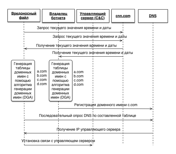
In general, a malicious file needs a seed to initialize a pseudo-random number generator (PRNG). The seed can be any parameter that will be known to the malicious file and the owner of the botnet. In our case, this is the value of the current date and time taken from the cnn.com resource. Using the same initialization vectors, the malicious file and the botnet owner get identical domain name tables. After that, the botnet owner only needs to register one domain in order for the malicious file, recursively sending requests to the DNS server, to get the IP address of the management server for further connection with it and receiving commands.
Recognition
Currently, there are many works related to the analysis of domain name generation algorithms. Some of them use Machine Learning methods. In general, the well-known models that can be found in the processing and analysis environment of natural languages are used — the models n-gramm, TF-IDF, etc.
However, the question arises of the training set. Our sample will consist of 2 classes. The first, Legit, was taken from the Alexa Top Million list. The second, DGA, was compiled by reverse engineering algorithms for generating malicious domain names taken from malware instances on the Internet, and is available in the repository ( https://github.com/andrewaeva/DGA ).
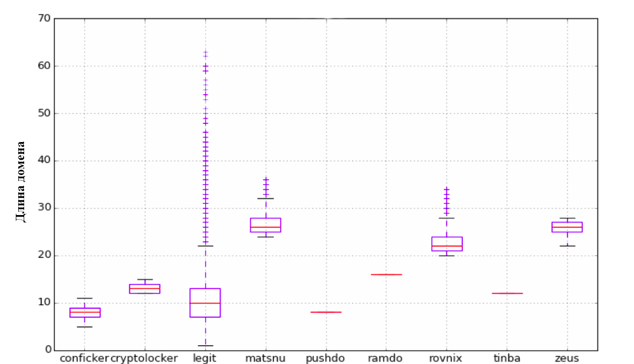
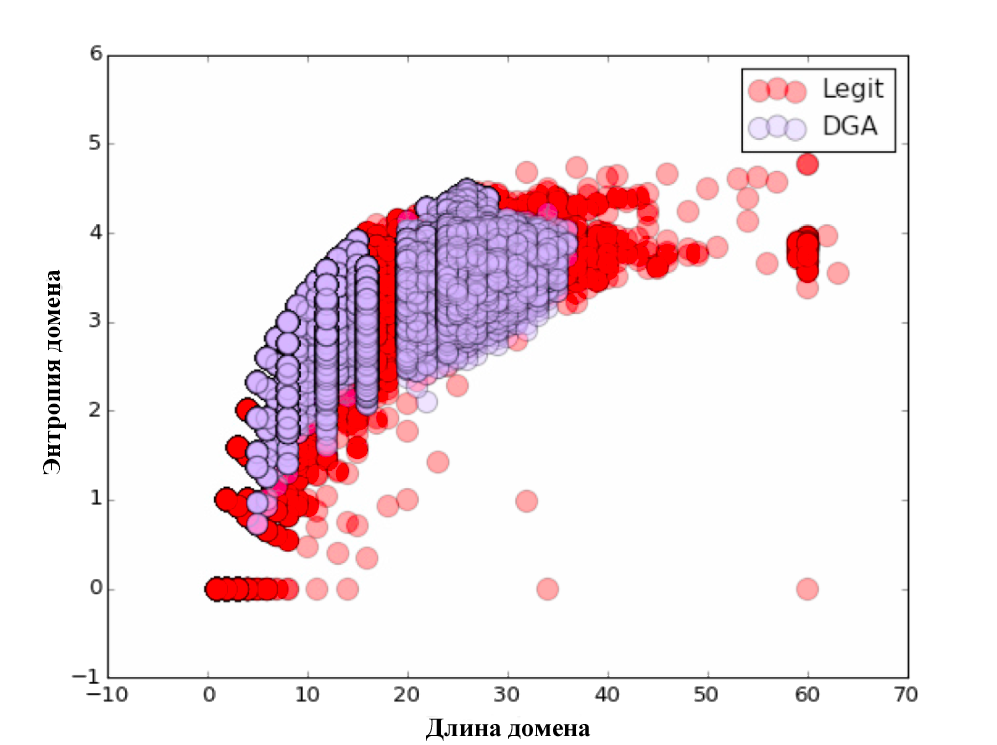
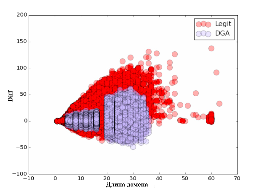
To begin with, we tried the approach described by the guys from licksecurity. They propose using the following list of parameters: length, entropy, TF-IDF model with N-gram selection. The first parameter is the length of the domain name. The second parameter is entropy. Further, the N-gram model was considered. Each n-gram (from 3 to 5) was represented as a vector in n-dimensional space, and the distance between them was calculated using the scalar product of these vectors. This is quite simply implemented using the Scikit Learn library.
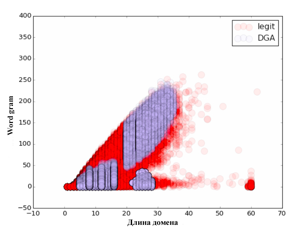
import numpy as np from sklearn.feature_extraction.text import CountVectorizer alexa_vc = CountVectorizer(analyzer='char', ngram_range=(3, 5), min_df=1e-4, max_df=1.0) counts_matrix = alexa_vc.fit_transform(dataframe_dict['alexa']['domain']) alexa_counts = np.log10(counts_matrix.sum(axis=0).getA1()) dict_vc = CountVectorizer(analyzer='char', ngram_range=(3, 5), min_df=1e-5, max_df=1.0) counts_matrix = dict_vc.fit_transform(word_dataframe['word']) dict_counts = np.log10(counts_matrix.sum(axis=0).getA1()) all_domains['alexa_grams'] = alexa_counts * alexa_vc.transform(all_domains['domain']).T all_domains['word_grams'] = dict_counts * dict_vc.transform(all_domains['domain']).T all_domains['diff'] = all_domains['alexa_grams'] - all_domains['word_grams'] As a result, we received an additional 3 parameters: Alexa gram — cosine distance to a dictionary consisting of the Alexa Top Million domains; Word gram — cosine distance to a specially composed dictionary consisting of the most commonly used words and phrases; and diff = alexa gram - word gram .
For each of the parameters we have built visual charts. Do not forget to look :)

The classification itself was carried out on the 80/20 principle, i.e. training took place on 80% of the initial data, and the testing of the algorithm on the remaining 20%. After checking the quality of the classification, the following results were obtained:
| Algorithm | Classification accuracy |
|---|---|
| Logistic regression | 87% |
| Random forest | 95% |
| Naive bayes | 75% |
| Extra tree forest | 94.6% |
| Voting Classification | 94.7% |
We thought, why so far no one has tried to use neural networks? Need to try!
Neural networks
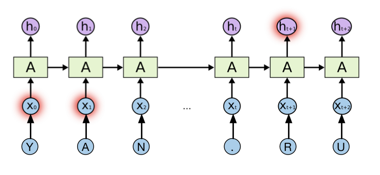
To solve our problem, we used a recurrent neural network. Recurrent neural networks are mainly characterized by the presence of a cycle. They allow you to save and use the information obtained from the previous steps of the neural network. In our case, each domain is considered as a sequence of characters from a fixed dictionary, which is fed to the input of a recurrent neural network. Training of such a neural network is carried out by the method of back propagation of an error in such a way as to maximize the probability of the correct choice of the corresponding class.
Recurrent neural network and Yandex.ru
Such a neural network architecture can analyze information that was previously submitted for data analysis at the current time. However, in practice it turns out that if the gap between the past information and the present is large enough, then this connection is lost, and such a network is unable to process it. A solution to this problem was found in 1997 by Hochreiter & Schmidhuber scientists. In their work, they proposed a new model of the recurrent neural network, namely the Long short-therm memory. Currently, this model is widely used to solve various classes of tasks, such as: speech recognition, processing of natural languages, etc. LSTM consists of a number of constantly connected subnets known as memory blocks. Instead of a single layer of the neural network, this model uses 4 layers that interact in a special way. In our model, we will use a variation of the LSTM model, namely the Gated Recurrent Unit (GRU). You can read more about LSTM and GRU in a wonderful article ( http://colah.imtqy.com/posts/2015-08-Understanding-LSTMs/ ), and we will move on.
To implement our model, we will use Python and all the favorite libraries of Theano ( https://pypi.python.org/pypi/Theano ) and Lasagne ( https://pypi.python.org/pypi/Lasagne/0.1 ).
Let's load our data into memory (yes, we are lazy) and do the preprocessing:
import numpy as np import pandas as pd import theano import theano.tensor as T import lasagne dataset = pd.read_csv('/home/andrw/dataset_all_2class.csv', sep = ',') dataset.head() chars = dataset['domain'].tolist() chars = ''.join(chars) chars = list(set(chars)) print chars # ['-', '.', '1', '0', '3', '2', '5', '4', '7', '6', '9', '8', '_', 'a', 'c', 'b', 'e', 'd', 'g', 'f', 'i', 'h', 'k', 'j', 'm', 'l', 'o', 'n', 'q', 'p', 's', 'r', 'u', 't', 'w', 'v', 'y', 'x', 'z'] classes = dataset['class'].tolist() classes = list(set(classes)) print classes #['dga', 'legit'] Now we will encode our domain into a sequence and form arrays X, y, mask M. Why do we need a mask? It's simple, Carl! Domains of varying length.
char_to_ix = { ch:i for i,ch in enumerate(chars) } ix_to_char = { i:ch for i,ch in enumerate(chars) } class_to_y = { cl:i for i,cl in enumerate(classes) } NUM_VOCAB = len(chars) NUM_CLASS = len(classes) NUM_CHARS = 75 N = len(dataset.index) X = np.zeros((N, NUM_CHARS)).astype('int32') M = np.zeros((N, NUM_CHARS)).astype('float32') Y = np.zeros(N).astype('int32') for i, r in dataset.iterrows(): inputs = [char_to_ix[ch] for ch in r['domain']] length = len(inputs) X[i,:length] = np.array(inputs) M[i,:length] = np.ones(length) Y[i] = class_to_y[r['class']] Form a training and test sample:
rand_indx = np.random.randint(N, size=N) X = X[rand_indx,:] M = M[rand_indx,:] Y = Y[rand_indx] Ntrain = int(N * 0.75) Ntest = N - Ntrain Xtrain = X[:Ntrain,:] Mtrain = M[:Ntrain,:] Ytrain = Y[:Ntrain] Xtest = X[Ntrain:,:] Mtest = M[Ntrain:,:] Ytest = Y[Ntrain:] Now everything is ready to describe the architecture of our network, which looks like the one shown in the figure. For classification, we will transfer the state of the last hidden layer to the Softmax layer, the output of which we can interpret as the probabilities of a domain belonging to one of the classes (malicious or legitimate).

BATCH_SIZE = 100 NUM_UNITS_ENC = 128 x_sym = T.imatrix() y_sym = T.ivector() xmask_sym = T.matrix() Tdata = np.random.randint(0,10,size=(BATCH_SIZE, NUM_CHARS)).astype('int32') Tmask = np.ones((BATCH_SIZE, NUM_CHARS)).astype('float32') l_in = lasagne.layers.InputLayer((None, None)) l_emb = lasagne.layers.EmbeddingLayer(l_in, NUM_VOCAB, NUM_VOCAB, name='Embedding') l_mask_enc = lasagne.layers.InputLayer((None, None)) l_enc = lasagne.layers.GRULayer(l_emb, num_units=NUM_UNITS_ENC, name='GRUEncoder', mask_input=l_mask_enc) l_last_hid = lasagne.layers.SliceLayer(l_enc, indices=-1, axis=1, name='LastState') l_softmax = lasagne.layers.DenseLayer(l_last_hid, num_units=NUM_CLASS, nonlinearity=lasagne.nonlinearities.softmax, name='SoftmaxOutput') output_train = lasagne.layers.get_output(l_softmax, inputs={l_in: x_sym, l_mask_enc: xmask_sym}, deterministic=False) total_cost = T.nnet.categorical_crossentropy(output_train, y_sym.flatten()) mean_cost = T.mean(total_cost) #accuracy function argmax = T.argmax(output_train, axis=-1) eq = T.eq(argmax,y_sym) acc = T.mean(eq) all_parameters = lasagne.layers.get_all_params([l_softmax], trainable=True) all_grads = T.grad(mean_cost, all_parameters) all_grads_clip = [T.clip(g,-1,1) for g in all_grads] all_grads_norm = lasagne.updates.total_norm_constraint(all_grads_clip, 1) updates = lasagne.updates.adam(all_grads_norm, all_parameters, learning_rate=0.005) train_func_a = theano.function([x_sym, y_sym, xmask_sym], mean_cost, updates=updates) test_func_a = theano.function([x_sym, y_sym, xmask_sym], acc We train our model by breaking the sample into batches of 100 domain names. As a result, we get the following graph:
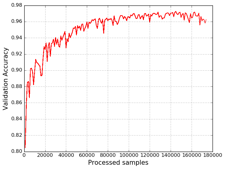
In conclusion, we can say that the resulting model is not at all inferior to the Random Forest algorithm, and even surpasses it. In addition, our model can be further improved, for example, by adding a reverse pass through the domain name to it or by including an attention mechanism (Attention LSTM) in the model. Well, for the topic of machine learning in information security, everything is just beginning :)
References
- https://github.com/ClickSecurity/data_hacking/blob/master/dga_detection/DGA_Domain_Detection.ipynb
- http://colah.imtqy.com/posts/2015-08-Understanding-LSTMs/
- https://github.com/andrewaeva/DGA/
- http://openbooks.ifmo.ru/ru/collections_article/997/raspoznavanie_i_klassifikaciya_vredonosnyh_domennyh_imen.html
- http://openbooks.ifmo.ru/ru/collections_article/4053/analiz_algoritmov_generacii_vredonosnyh_domennyh_imen_i_metody_ih_raspoznavaniya_s_ispolzovaniem_rekurrentnyh_neyronnyh_setey.hht
Abakumov Andrey, Digital Security
Source: https://habr.com/ru/post/282433/
All Articles