R: Geospatial Libraries

Input / output, modification and visualization of geospatial data are tasks common to many disciplines. Therefore, many are interested in creating good tools to solve them. A set of tools for working with spatial data is constantly growing. We superficially consider each of them. Details can be obtained via links to cran or github .

We are not trying to replace the geospatial libraries that already exist in R — rather, to supplement and create small tools that make it easy to use only the functions you need.

geojsonio

cran github

geojsonio is a tool for converting data from and to geojson format. Convert data to / from GeoJSON from various R classes: vectors, lists, data frames, vector files, and spatial classes.
')
For example:

library("geojsonio") geojson_json(c(-99.74, 32.45), pretty = TRUE) 

 #> { #> "type": "FeatureCollection", #> "features": [ #> { #> "type": "Feature", #> "geometry": { #> "type": "Point", #> "coordinates": [-99.74, 32.45] #> }, #> "properties": {} #> } #> ] #> } 

wellknown

cran github

wellknown is a tool for converting to and from text data in a well-known format. Convert WKT / WKB to GeoJSON and back. Included are functions for converting between GeoJSON and WKT / WKB, creating GeoJSON properties, creating WKT / WKB from R objects (for example, lists, data frames (data frame), vectors), WKT assemblies.

For example:

 library("wellknown") point(data.frame(lon = -116.4, lat = 45.2)) 

 #> [1] "POINT (-116.4000000000000057 45.2000000000000028)" 

gistr

cran github

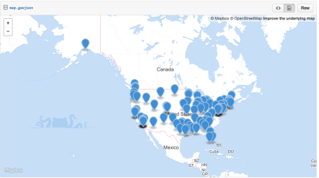
The gistr is not a geospatial tool in and of itself, but it is extremely useful for sharing maps. Say, with just a few lines, you can share an interactive map on GitHub.

For example, using the geojsonio described above:

 library("gistr") cat(geojson_json(us_cities[1:100,], lat = 'lat', lon = 'long'), file = "map.geojson") gist_create("map.geojson") 

lawn

cran github

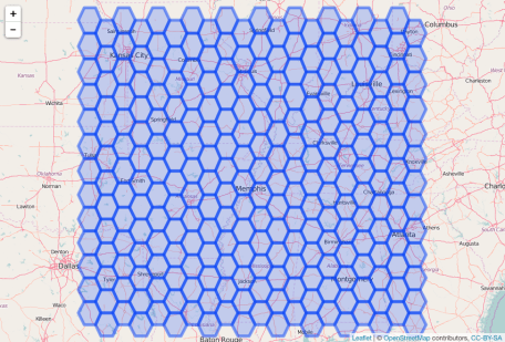
R-client for turf.js ( advanced geospatial analysis for browsers and modules ).

In lawn there is a function for each method in turf.js And:

• several wrapper functions for the modular geojson-random package (creating random geojson properties);
• auxiliary function view() for easy visualization of the results of calling lawn functions.

For example:

 library("lawn") lawn_hex_grid(c(-96,31,-84,40), 50, 'miles') %>% view 

geoaxe

cran github

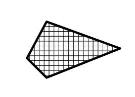
R client for splitting geospatial objects into parts.

For example:

 library("geoaxe") library("rgeos") wkt <- "POLYGON((-180 -20, -140 55, 10 0, -140 -60, -180 -20))" poly <- rgeos::readWKT(wkt) polys <- chop(x = poly) plot(poly, lwd = 6, mar = c(0, 0, 0, 0)) 

And the polyhedron divided into parts:

 plot(polys, add = TRUE, mar = c(0, 0, 0, 0)) 

proj

cran github

R-client for proj4js , Javascript-library for projections. proj is not on CRAN yet.

getlandsat

cran github

R-client for Landsat data from AWS public repositories. getlandsat not yet on CRAN.

For example:

 library("getlandsat") head(lsat_scenes()) 

 #> entityId acquisitionDate cloudCover processingLevel #> 1 LC80101172015002LGN00 2015-01-02 15:49:05 80.81 L1GT #> 2 LC80260392015002LGN00 2015-01-02 16:56:51 90.84 L1GT #> 3 LC82270742015002LGN00 2015-01-02 13:53:02 83.44 L1GT #> 4 LC82270732015002LGN00 2015-01-02 13:52:38 52.29 L1T #> 5 LC82270622015002LGN00 2015-01-02 13:48:14 38.85 L1T #> 6 LC82111152015002LGN00 2015-01-02 12:30:31 22.93 L1GT #> path row min_lat min_lon max_lat max_lon #> 1 10 117 -79.09923 -139.66082 -77.75440 -125.09297 #> 2 26 39 29.23106 -97.48576 31.36421 -95.16029 #> 3 227 74 -21.28598 -59.27736 -19.17398 -57.07423 #> 4 227 73 -19.84365 -58.93258 -17.73324 -56.74692 #> 5 227 62 -3.95294 -55.38896 -1.84491 -53.32906 #> 6 211 115 -78.54179 -79.36148 -75.51003 -69.81645 #> download_url #> 1 https://s3-us-west-2.amazonaws.com/landsat-pds/L8/010/117/LC80101172015002LGN00/index.html #> 2 https://s3-us-west-2.amazonaws.com/landsat-pds/L8/026/039/LC80260392015002LGN00/index.html #> 3 https://s3-us-west-2.amazonaws.com/landsat-pds/L8/227/074/LC82270742015002LGN00/index.html #> 4 https://s3-us-west-2.amazonaws.com/landsat-pds/L8/227/073/LC82270732015002LGN00/index.html #> 5 https://s3-us-west-2.amazonaws.com/landsat-pds/L8/227/062/LC82270622015002LGN00/index.html #> 6 https://s3-us-west-2.amazonaws.com/landsat-pds/L8/211/115/LC82111152015002LGN00/index.html 

siftgeojson

cran github

Make GeoJSON slices as easy as you would with a data frame. This is a superstructure over jqr , R-wrappers for jq , a JSON handler.

 library("siftgeojson") #    file <- system.file("examples", "zillow_or.geojson", package = "siftgeojson") json <- paste0(readLines(file), collapse = "") #     (Multnomah), ,      (Multnomah) sifter(json, COUNTY == Multnomah) %>% jqr::index() %>% jqr::dotstr(properties.COUNTY) 

 #> [ #> "Multnomah", #> "Multnomah", #> "Multnomah", #> "Multnomah", #> "Multnomah", #> "Multnomah", #> "Multnomah", #> "Multnomah", #> "Multnomah", ... 

plotly

cran github

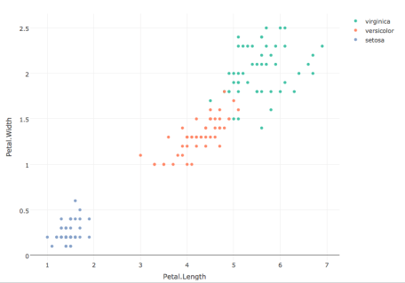
plotly - R-client for Plotly - a web-based interface and API for creating interactive graphics.

 library("plotly") plot_ly(iris, x = Petal.Length, y = Petal.Width, color = Species, mode = "markers") 

Maptools Task View

github

Jeff Hollister created the maptools task view to organize work with maps in R: packages, data sources, projections, static and interactive maps, data transformations, etc.