From idea to development: what you need to know about creating strategies for trading on the exchange. Part III

On Habré and in the analytical section of our site, we write a lot about financial market trends and continue to publish a series of materials on creating strategies for trading on the stock exchange, based on the articles of the author of the blog Financial Hacker. In the previous materials, revealing the main theses of the cycle of articles by the author of the blog Financial Hacker, we talked about using market inefficiencies on the example of a history with a price limit for the Swiss franc and considered important factors that need to be considered when creating strategies for trading on the stock exchange.
This time we will discuss the general principles for the development of model-oriented trading systems.
')
Developing an "ideal" strategy
As in many other cases, when it comes to developing strategies for trading on the stock exchange, there are two ways: the ideal and the real. To begin, consider the ideal process of developing a strategy.
Step 1. Selecting a model
To begin with, a trader should choose one of the previously described market inefficiencies or discover a new one. It is possible that some ideas will appear in the analysis of the price curve, when something suspicious will meet a certain logic of the market. The opposite variant is also suitable - from the theory of behavioral pattern to its verification on real data. True, all the laws and inefficiencies are likely to have already been discovered and studied by other market participants for many years.
Having defined the model, it will be necessary to choose a price anomaly that corresponds to it. Then, describe it using a quantitative formula or, in extreme cases, by means of a qualitative criterion. As an example, you can use the cyclic model from the previous article:

In our case, (Ci) is the duration, (Di) is the phase and (ai) is the amplitude. One of the most successful foundations in history, Renaissance Medallion, says that it was able to achieve good results using the cycle model along with the hidden Markov model.
Step. 2. Searches
It is also necessary to make sure that the chosen anomaly really manifests itself in the price curve of the assets with which the trader is going to trade. This can be checked with the help of historical data - D1, M1 and tick values, showing the distribution of the anomaly along the time axis. The whole question is, how deep into the past do you need to dig? Answer: as far as possible. Until the conditions for the occurrence of anomalies are clarified. Then you have to write a script that will find and demonstrate an anomaly on the price curve. In our example, this will be the frequency spectrum for the euro / dollar pair:
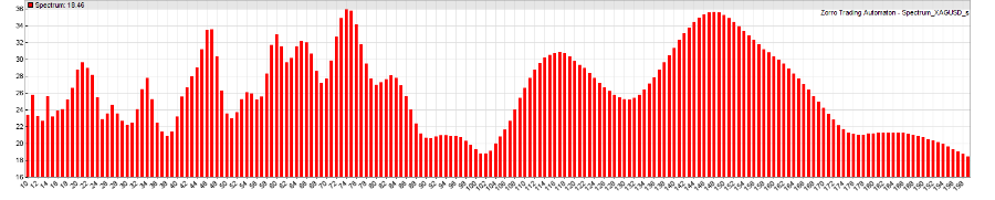
It is necessary to find out how the spectrum changes for arbitrary periods of time - months and years, and then compare it with the spectrum of random data (in some programming languages, like Zorro, there are special functions for randomizing curves). If no signs of anomaly and differences from the random distribution are found, the trader will have to improve the method of detecting the anomaly. And if nothing happens - then go back to step 1.
Step 3. Algorithm
The next step involves writing an algorithm that will generate trading signals for opening and closing positions, following the chosen anomaly. In a typical situation, market inefficiency has little effect on the price curve. Therefore, the algorithm must be finely tuned to separate the manifestation of the anomaly from random noise. At the same time, it should be as simple as possible, and based on the minimum number of free parameters. In our version, the script changes the position on each trough and peak of the sinusoid that goes over the dominant cycle:
function run() { vars Price = series(price()); var Phase = DominantPhase(Price,10); vars Signal = series(sin(Phase+PI/4)); if(valley(Signal)) reverseLong(1); else if(peak(Signal)) reverseShort(1); } This is the core of the system. Now it's time to backtest. The accuracy of the execution of the task in this case is not so important, you just need to determine the limits of the algorithm. Can he make a series of lucrative deals in specific market situations? If not, there are two options: rewrite or re-create using another method. At this stage, it is not necessary to stuff the algorithm with trailing stops and other stuffing. They will distort the result and create the illusion of profit from scratch. The algorithm must learn to just make a profit, at least in the case of closing positions in time.
At this stage, you also need to determine the data for the backtest. For a working test, M1 and tick quotes are sufficient. Daily data is not suitable. The amount of data depends on the duration of the anomaly (which was determined at the second stage) and its nature. Usually, the longer the period, the more accurate the test. It makes no sense to dig deeper than 10 years. At least, if we are talking about real-life market behavior, in a dozen years the market has changed critically. Outdated data will give incorrect results.
Step 4. Filter
No inefficiency lasts forever. Any market goes through periods of arbitrary behavior of quotes. Therefore, for each successful trading system is critical to have a filter that would determine the presence or absence of inefficiency. The filter is just as important as the signal, if not more important. But, for various reasons, he is often forgotten. Below is an example of a script installing a filter for a trading system:
function run() { vars Price = series(price()); var Phase = DominantPhase(Price,10); vars Signal = series(sin(Phase+PI/4)); vars Dominant = series(BandPass(Price,rDominantPeriod,1)); var Threshold = 1*PIP; ExitTime = 10*rDominantPeriod; if(Amplitude(Dominant,100) > Threshold) { if(valley(Signal)) reverseLong(1); else if(peak(Signal)) reverseShort(1); } } Here a bandpass filter is applied, centered on the period of the dominant cycle to the price curve and measuring its amplitude. If the amplitude exceeds the set limit, then you can be sure that there is inefficiency and act accordingly. The duration of the transaction is now also limited to a maximum of 10 cycles, since at the second stage we found out that the dominant cycle appears and disappears in relatively short time intervals.
What could go wrong here? An error will add a filter simply because it improves the test result. Any filter should have a rationale behind it, building on market behavior or algorithm signals.
Step 5. Optimization of parameters
All system parameters, one way or another, affect the result. But only a few of them directly determine entry and exit points based on the price curve. It is necessary to identify and optimize these adaptable parameters. In our example, the opening position is determined by the phase of predicting the behavior of the curve and the threshold set by the filter. The closing time is determined by the exit point. Other parameters, such as the DominantPhase filter constant and the BandPass function, need to be optimized, since their values do not depend on the market situation.
Often the optimization is interpreted incorrectly. The method of genetic or forced optimization is an attempt to find the peak of gain in a multidimensional parameter space. In most cases, this is not related to the work of a living system. Although it may turn out a unique combination of parameters, which will give an excellent test result. Even quite a bit different historical periods give completely different peaks. Instead of chasing the value of the maximum profit on the historical curve, optimization should go the following way:
- It can determine the sensitivity of the system to parameter values. If the system misses its boundaries with minimal changes in parameters, it is better to return to step 3. If the situation cannot be rectified, go back to the first stage.
- Through optimization, you can find the active points of the parameters. This is the zone where the parameters are most reliable, that is, where even a small change does not have a significant effect on a positive result. These are not narrow peaks, as one might think, but wide hills in the parameter space.
- It can adapt the system to various assets and allow working with a portfolio of stocks with minimal changes in parameters.
- It can increase the service life of the system through the adaptation of parameters to the current market situation at regular intervals, in parallel with the process of "live" trading.
Here is an example script for optimizing parameters:
function run() { vars Price = series(price()); var Phase = DominantPhase(Price,10); vars Signal = series(sin(Phase+optimize(1,0.7,2)*PI/4)); vars Dominant = series(BandPass(Price,rDominantPeriod,1)); ExitTime = 10*rDominantPeriod; var Threshold = optimize(1,0.7,2)*PIP; if(Amplitude(Dominant,100) > Threshold) { if(valley(Signal)) reverseLong(1); else if(peak(Signal)) reverseShort(1); } } The two optimized calls use a starting value of 1.0 and a range (0.7..2.0) to determine the active points of the two main parameters. In the profit chart, these points are marked with red columns:
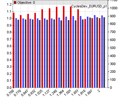
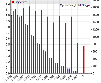
In this embodiment, the optimizer chooses a parameter value close to 1.3 for the sinusoid phase and a value of 1.0 (not 0.9 for the peak) for the threshold amplitude for the current ratio in the euro / dollar pair. The exit time is not optimized here.
Step 6. Analysis outside the sample.
Parameter optimization improves the quality of the verification test. But our system is still not fitted to the price curve. Therefore, the test results for now are useless. Now you need to divide the data into cycles in the sample and beyond. The sample is used for training the system, the analysis outside the sample is used for testing. The standard method for this is forward analysis . It uses dynamic sampling or a sliding window for historical data to separate the two cycles.
Unfortunately, forward analysis adds two new parameters to the system: training time and testing time. The second is not critical, as long as it is relatively small. But learning time matters. Too short training will not allow to get enough data at a price for effective optimization. Too long will also negatively affect the result. The market may already “digest” changes while it is being trained. Therefore, the learning time itself needs to be optimized.
Forward analysis in increments of five cycles (set NumWFOCycles = 5 in the previous script) reduces the backtest performance from 100% of annual revenue to a more realistic 60%. In order to avoid too optimistic results and errors in the analysis, you can run it several times with slightly different simulation conditions. If the system has its limits, the results should not be too different. Otherwise, you will need to return to step 3.
Step 7. Test the reality
Even after passing the stage of analysis outside the sample, we still have some distortion of the result. Are they caused by a limitation of the system itself or by shortcomings in the development process (asset selection, algorithm, verification time, and so on)? Finding this out is the hardest part in working on a trading strategy.
The best option is to use for this purpose a method called Testing Reality According to White’s Reality Check. It is also the least practical, as it requires a strict order in the choice of parameters and algorithm. Two other methods are not so good, but more convenient to use:
- Monte Carlo . It assumes randomization of the price curve by shuffling the data without changing them. Then you need to train the system and test it again, and then do it all over again and generate the distribution of results. Randomization will remove all price anomalies. But if the result of the real price curve is not so far from the peak of the random distribution, it is probably also caused by chance. What does it mean? Need to go back to step 3.
- Variants . This method is the opposite of the previous one. It adapts the learning system to different variants of the price curve in order to get a positive result. Variants that support most anomalies are sampled at an increased frequency, eliminate the influence of a trend, or invert the price curve. If the system is to win with such options, but not with random prices, you really picked up something worthwhile.
- ROOS test (Really-out-of-sample) . This implies a complete exclusion in the process of developing data for the last year (in the example, 2015), up to the removal of data on price movements from a computer. And only when the system is fully completed, you need to download data for this year and run the test. Here you will need to gather all the will into a fist in order not to become a remake of the system if it does not show the desired results on this latest test. You just need to set it aside and return to step 1.
Step 8. Risk Management
So, the system has gone through all the checks. Now you can focus on reducing risk and increasing its productivity. You no longer need to return to the input data of the algorithm and its parameters. It is necessary to optimize what will be obtained at the output. Instead of a simple time limit and cancellation, you can use mechanisms of various trailing stops to exit. For example:
- Instead of exiting after a predetermined period of time, you need to set the stop loss to the loss value for each hour. The effect will be similar, but now closing of unsuccessful transactions will be faster, and successful later.
- Stop loss should be placed when a certain profit value is reached above the rollback point of values. Even if fixing a profit percentage does not improve overall performance, it will still be useful.
Here is an example of a script that sets stop loss:
function run() { vars Price = series(price()); var Phase = DominantPhase(Price,10); vars Signal = series(sin(Phase+optimize(1,0.7,2)*PI/4)); vars Dominant = series(BandPass(Price,rDominantPeriod,1)); var Threshold = optimize(1,0.7,2)*PIP; Stop = ATR(100); for(open_trades) TradeStopLimit -= TradeStopDiff/(10*rDominantPeriod); if(Amplitude(Dominant,100) > Threshold) { if(valley(Signal)) reverseLong(1); else if(peak(Signal)) reverseShort(1); } } Of course, now we have to go through the optimization process and forward analysis for the output parameters.
Step 9. Distribution of funds
The process of managing funds has three objectives. First, reinvest income. Secondly, correctly distribute the capital within the portfolio. Thirdly, in time to understand that the trading portfolio is useless. In any textbook on trading, you can find advice to invest 1% of the total capital per transaction. These things are written by people who have not earned a cent in real trading.
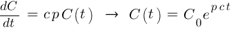
We denote the volume of investment in a fixed time by V (t). If the system generates revenue, on average, capital C will grow proportionally with a factor c.
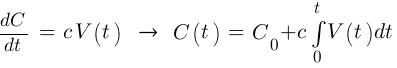
If you follow the advice of authors of smart books and invest a fixed percentage of p on capital, V (t) = p C (t), then capital should grow by the exponent p c.
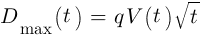
Unfortunately, at the same time, capital will experience the effects of random fluctuations. Such drawdowns will be proportional to the volume of funds traded V (t). This can be calculated using the formula where the maximum depth of drawdown D max will increase in proportion to the square root of t.
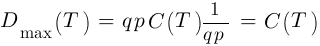
Thus, with a fixed value of investment we get:

And time in this case is T = 1 / (qp) 2
From these calculations, you can see how, during period T, the drawdown will eat all the money in the account. It does not matter how good the trading system itself is, and what percentage of the investment the trader set. Therefore, the advice “to invest 1% at a time” is bad advice. That is why the author of the blog Financial Hacker advises its customers not to increase the trading volume proportionally to the accumulated profit, but to do so by the square root. Until the strategy itself is exhausted, it will keep the trader at a safe distance from the margin call .
Depending on whether the trader works with one asset and one algorithm or with their sets, the optimal amount of investment can be calculated by several methods. For example, according to the OptimalF formula of Ralph Vince or according to the Kelly formula from Ed Thorpe. In most cases, it is logical to move away from the ponderous code to implement the reinvestment process, so the amount of investment can be calculated outside the algorithm. Especially if the trader is going to withdraw or deposit money into the account from time to time. A convenient formula for such things can be found in the manual for the language Zorro .
Step 10. Preparing for real trading
It's time to decide on the user interface for the trading system. To do this, it is necessary to understand which parameters will need to be changed in real time, and which ones will remain constant. Next, you should adapt the trading volume management method to it and implement a “panic button” for recording profits and going to the cache when bad news appears. It is necessary to display all the essential parameters of trading in real time, add opportunities for retraining the system and include in it a method of checking real results with backtest results. The trader must make sure that he can control the system from any point in space and time. This does not mean that it should be checked every five minutes. But to have the opportunity at lunch to look at the results of trading with a mobile phone never hurts.
As all often happens in reality
Above, we described the development of an ideal strategy. It all looks pretty. But how to develop a real trading strategy? It is clear that there is a gulf between theory and practice - which, of course, is wrong.
Here is how often the sequence of steps to create a strategy of work on the exchange, which is done by hundreds and thousands of traders:
Step 1 . Go to the forum of traders and get a hint about a new steep indicator, which brings fabulous revenues.
Step 2 . To torment yourself with the test system code to make sure that the indicator is working. The backtest results are not impressive? An error has crept into the code. It is necessary to make debugging, to try even better.
Step 3 . There is still no result, but the trader is already aware that he has mastered several useful moves. You can also add a trailing stop. Now everything looks a little better. It's time to start the weekly analysis. Tuesday falls out of strategy? You need to add a filter that skips trading on Tuesdays. Add a few more filters that block the opening of positions between 10 and 12 in the morning, if the quote is less than $ 14.5, and during the full moon period. Wait for the simulation to complete. Great, the backtest results are good now!
Step 4 . Of course, no one is conducted simply on the result of the sample. After optimizing all 23 parameters, the trader starts the forward analysis. Is waiting. Do not like the result? He tries different cycles of this analysis, different periods. Still waiting. Finally, the desired values will appear.
Step 5 . The system is launched during real trading.
Step 6 . The result does not look impressive.
Step 7 . After the fiasco it remains only to wait until the bank account comes to life. Some traders in such periods are engaged in writing books on trading on the stock exchange.
In the following material, we will look at the approach of using data mining techniques in combination with machine learning to detect patterns using various algorithms and neural networks.
Source: https://habr.com/ru/post/281148/
All Articles